How LLMs Work, Part 3: From Toy Model to GPT
How LLMs Work, Part 3: From Toy Model to GPT
In Part 1 I covered how text gets tokenized, embedded, and processed through the transformer architecture. In Part 2 I went through backpropagation, gradient descent, and the Adam optimizer. But there is a massive gap between a toy model that trains in seconds on a laptop and models like Llama 3 that train on thousands of GPUs for weeks. In this article I go through memory, parallelism, and training cost first, then what the model actually learns at different layers, and finally the post-training steps like fine-tuning and RLHF that turn a raw model into a usable assistant.
Scaling: What Changes When You Go from Toy to GPT
The Problem: One GPU Is Not Enough
The toy model from Part 2 fits in a few megabytes and trains in seconds. Real LLMs need significantly more.
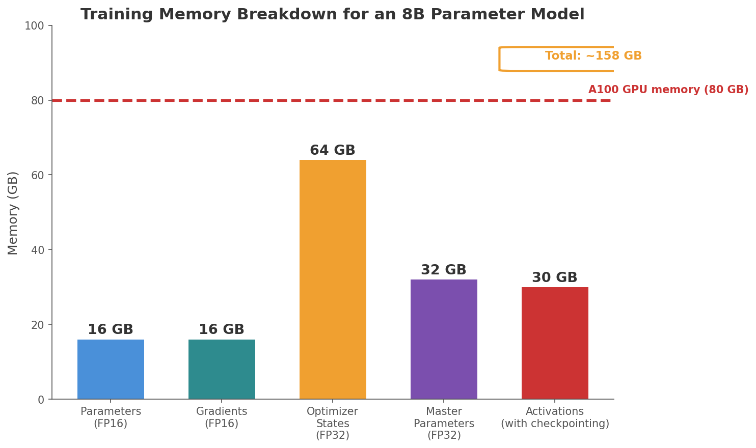
Llama-3.1-8B has 8 billion parameters. As I discussed in the TurboQuant post, each parameter stored in FP16 (16-bit floating point) takes 2 bytes. So just storing the model parameters takes 8 billion x 2 bytes = 16 GB.
But during training, you need much more than just the parameters:
- Gradients: one gradient value for each parameter. Same size as the parameters: 16 GB.
- Optimizer states: Adam stores two extra values per parameter (the momentum and the squared gradient running averages). These are kept in FP32 (4 bytes each) for numerical precision. That is 8 billion x 4 bytes x 2 = 64 GB.
- Activations: the intermediate outputs of each layer. During the forward pass, every layer takes an input, transforms it, and produces an output. That output has to be stored in memory because backpropagation needs it later. In the toy example from Part 2, when we computed the gradient for
w3, we needed the value ofa = -0.3, which was computed during the forward pass. If we had not storeda, we would have had to recompute the entire forward pass up to that point just to get one gradient. Scaling that up to a real model with 32 layers, every layer produces intermediate outputs, and every one of those outputs needs to be kept in memory until backpropagation reaches that layer working backwards. The total memory depends on batch size and sequence length. For Llama-3.1-8B with a batch of 1,024 sequences of 4,096 tokens: each token at each layer is represented as a 4,096-dimensional vector (the embedding dimension), and all 32 layers’ outputs need to be stored. That is 1,024 sequences × 4,096 tokens × 4,096 numbers per token × 32 layers × 2 bytes (FP16) ≈ 1 TB. Activation checkpointing brings this down significantly by not storing every layer’s output. Instead, some outputs are recomputed during backpropagation, trading computation time for memory savings.
On top of this, training uses mixed precision. The forward and backward passes run in FP16 (16-bit floating point) because GPUs are much faster at FP16 math. But FP16 can only represent about 3-4 significant digits. When Adam computes a tiny update like 0.000003 and adds it to a parameter like 1.234, FP16 rounds the result back to 1.234. The update is lost completely because it is too small for FP16 to represent. To avoid this, training keeps a master copy of every parameter in FP32 (32-bit, about 7 significant digits), which adds another 32 GB. The training loop copies parameters from FP32 to FP16 for the fast forward and backward pass, computes gradients in FP16, and then applies the Adam update to the FP32 master copy where the precision is high enough to accumulate small changes. Without the FP32 master, small gradient updates would get rounded away and the model would eventually stop learning.
The forward pass does use slightly imprecise FP16 values, but a small rounding error in the forward pass barely affects the gradient. What matters is the accumulation of updates over thousands of steps. A single update of 0.000003 disappears in FP16, but 10,000 such updates add up to 0.03 in FP32, which is significant.
Add it all up and training an 8B parameter model requires roughly 130 to 160 GB of memory (the exact number depends on the training setup and precision choices). A single NVIDIA A100 GPU has 80 GB. It does not fit.
For Llama-3.1-70B with 70 billion parameters, these numbers are roughly 9x larger. Training it requires many GPUs working together.
Data Parallelism
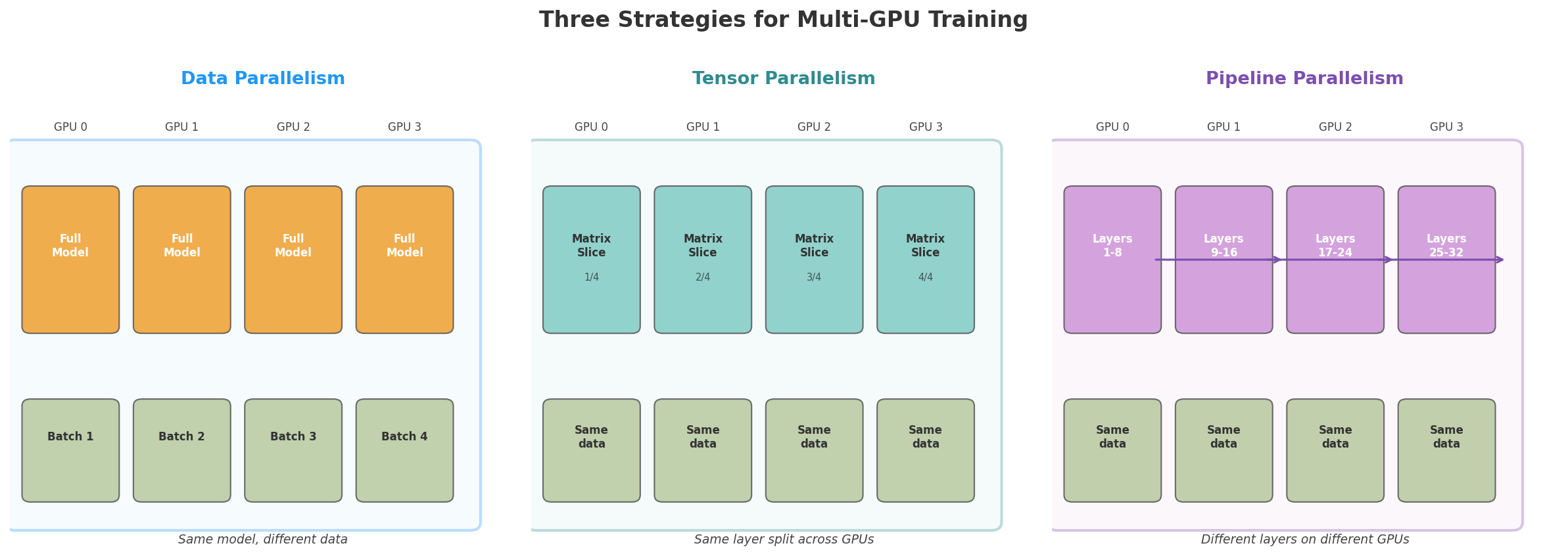
The simplest way to use multiple GPUs is to put a copy of the entire model on every GPU and give each GPU a different batch of data.
Each GPU runs the forward pass on its own batch, computes the loss, runs backpropagation, and gets its own gradients. Then the GPUs communicate to average their gradients using an operation called all-reduce, where each GPU sends its gradients and receives the averaged result. After averaging, every GPU has the same gradient values and applies the same update, so all copies of the model stay in sync.
This is called data parallelism. It speeds up training because you process N batches in parallel (one per GPU) in the time it would take to process one. With 8 GPUs, you get roughly 8x the throughput.
The limitation is that every GPU needs to hold the full model. If the model does not fit on one GPU, data parallelism alone is not enough.
Model Parallelism
When the model itself is too large for a single GPU, you split it across multiple GPUs.
Tensor parallelism splits individual parameter matrices (also called weight matrices) inside each layer across GPUs. For example, a 4,096 × 4,096 matrix could be sliced into four pieces of 4,096 × 1,024, with each piece on a different GPU. Each GPU gets the same input, multiplies it by its slice, and produces a partial result (1,024 numbers instead of 4,096). The GPUs then share and combine their partial results to get the full output. This requires fast interconnects between GPUs because the communication happens within every layer.
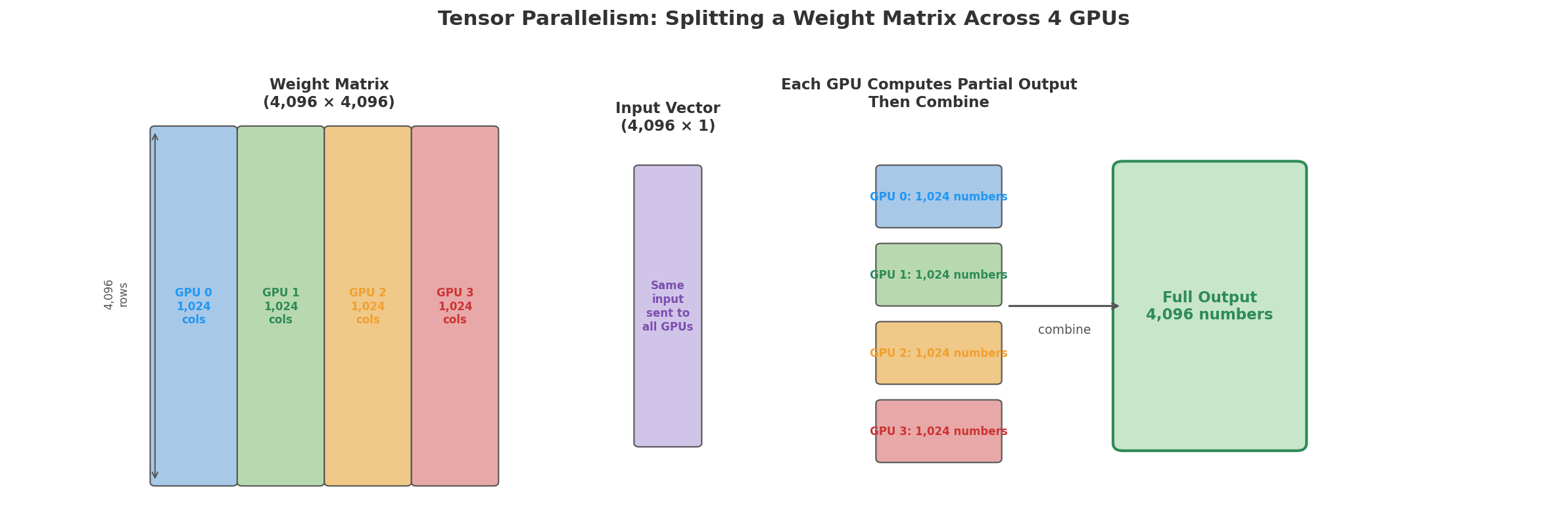
To see how this works, here is a small example. A 3×4 matrix multiplied by a 4-dimensional input:
Full multiplication (one GPU):

                  [ 1 ]
[ 2  1  3  0 ]   [ 2 ]     Row 0: (2×1)+(1×2)+(3×3)+(0×4) = 13
[ 0  4  1  2 ] × [ 3 ]  =  Row 1: (0×1)+(4×2)+(1×3)+(2×4) = 19
[ 1  0  2  3 ]   [ 4 ]     Row 2: (1×1)+(0×2)+(2×3)+(3×4) = 19
With tensor parallelism across 2 GPUs, split the matrix by columns. GPU 0 takes columns 0-1, GPU 1 takes columns 2-3. Each GPU multiplies its columns with the corresponding input elements:
GPU 0 (columns 0-1, input[0] and input[1]):
  Row 0: (2×1)+(1×2) = 4
  Row 1: (0×1)+(4×2) = 8
  Row 2: (1×1)+(0×2) = 1

GPU 1 (columns 2-3, input[2] and input[3]):
  Row 0: (3×3)+(0×4) = 9
  Row 1: (1×3)+(2×4) = 11
  Row 2: (2×3)+(3×4) = 18

Combine (add partial results): [4+9, 8+11, 1+18] = [13, 19, 19]
We got the same answer and each GPU did half the work and stores only half the weight matrix in its memory. In practice, the split direction varies by layer and sometimes the input gets split too, but the idea is the same.
Pipeline parallelism assigns different layers to different GPUs. GPU 1 handles layers 1 through 8, GPU 2 handles layers 9 through 16, and so on. Data flows from GPU 1 to GPU 2 to GPU 3 like an assembly line. While GPU 2 is processing batch 1, GPU 1 can start on batch 2. The downside is that there are “bubbles” where some GPUs sit idle waiting for data, but clever scheduling (like interleaving micro-batches) can reduce this waste.
In practice, large training runs use all three: data parallelism across groups of GPUs, tensor parallelism within each group, and pipeline parallelism across stages. Meta trained Llama 3 on 16,384 H100 GPUs using a combination of all three strategies.
The Cost of Training
Training compute is measured in FLOPs (floating point operations). A single FLOP is one arithmetic operation like a multiplication or an addition. A useful approximation from Kaplan et al. 2020 estimates the total FLOPs for training a transformer with N parameters on D tokens as roughly 6 * N * D.
The 6 comes from counting operations at each parameter. In a matrix multiplication, each output number is a sum of products. For example, with a 3-element input: output = (input[0] × w[0]) + (input[1] × w[1]) + (input[2] × w[2]). Take a single parameter like w[0]. In the forward pass, it does one multiply (input[0] × w[0]) and one add (adding that product to the running sum). That is 2 operations per parameter in the forward pass.
In the backward pass (covered in Part 2), the model works backward from the loss to figure out how to adjust each parameter. At each layer, it needs to answer two questions.
The first question is: how much did each parameter contribute to the error? During the forward pass, w[0] was multiplied by input[0]. To figure out how much w[0] affected the final error, the model multiplies the error signal (how wrong the output was) by input[0] (the value that w[0] was applied to). This is one multiply and one add per parameter.
The second question is: how much did the input to this layer contribute to the error? This is needed because the input came from the previous layer, and that layer also needs to know how to adjust its own parameters. To compute this, the model multiplies the error signal by w[0] itself (the parameter value). Another multiply and add per parameter.
That gives 4 operations per parameter in the backward pass (2 for the parameter gradient, 2 for the input gradient).
Combined: 2 (forward) + 4 (backward) = 6 operations per parameter per token. Multiply by N parameters and D tokens and you get 6 * N * D.
For Llama 2 70B: 6 × 70 billion × 2 trillion = 8.4 × 10²³ FLOPs.
Meta reported that Llama 2 70B used 1,720,320 GPU-hours on A100 GPUs (Touvron et al. 2023). The A100 is NVIDIA’s data center GPU with 80 GB of memory and 312 TFLOPS of BF16 compute, designed specifically for large-scale machine learning workloads. Meta used 2,048 A100 GPUs for Llama 2 70B, which works out to roughly 35 days of continuous training. Translating GPU-hours to dollar costs depends on whether you own the hardware or rent it, and at what rate. Estimates for larger proprietary models are speculative since training costs are not typically disclosed.
Chinchilla Scaling Laws
So far I covered how much memory and compute training requires. But given a fixed compute budget, is it better to train a larger model on less data, or a smaller model on more data?
The Chinchilla paper (Hoffmann et al. 2022) from DeepMind showed that for a given compute budget, there is an optimal balance between model size and data size. They found that, for a fixed training compute budget, model size and training tokens should scale together. A common rule of thumb from Chinchilla is about 20 training tokens per model parameter. A 10 billion parameter model should therefore train on roughly 200 billion tokens.
Before Chinchilla, the trend was to train very large models on relatively little data. GPT-3 had 175 billion parameters but trained on about 300 billion tokens. By the 20x rule, a model that large would train on about 3.5 trillion tokens, over 10x more data.
After Chinchilla, the field shifted toward training models on far more data. Llama 2 70B trained on 2 trillion tokens, above the 1.4 trillion suggested by the 20x rule. Llama 3 pushed much further: its 70B model trained on over 15 trillion tokens.
The practical implication is that, for a fixed compute budget, you are often better off training a smaller model on more data than a larger model on too little data. A well-trained smaller model can outperform an undertrained larger model.
Data Quality and Preprocessing
The raw data that goes into training is not clean. Common Crawl alone contains billions of web pages, and a large portion of them are spam, duplicate content, boilerplate text, or low-quality machine-generated text. Training on this data directly would produce a model that generates the same kind of noise.
A significant part of the training pipeline is data cleaning and filtering. Typical steps include deduplication, language identification, quality filtering, boilerplate removal, PII mitigation, and sometimes filtering or measuring toxic and harmful content. The original LLaMA paper describes preprocessing Common Crawl with the CCNet pipeline: deduplicating text, using fastText for language identification, filtering low-quality pages with an n-gram language model, and training a classifier to prefer pages similar to Wikipedia references. Llama 2 continued this general approach with a new public-data mix, more robust cleaning, and efforts to remove sources likely to contain large amounts of personal information.
The mix of data sources also matters. Training exclusively on web text produces a model that sounds like the internet. Mixing in books, scientific papers, code, and curated datasets like Wikipedia produces a more well-rounded model. The Pile dataset was specifically designed for this: it combines 22 different sources in carefully chosen proportions. Getting the data mix right is increasingly recognized as a first-order decision in LLM training, often as important as architecture or optimizer choices.
What the Model Actually Learns
After training on trillions of tokens, the model’s 8 billion parameters are no longer random. They encode patterns learned from the data. Researchers have been studying what exactly those patterns look like at each layer.
Layers Learn Different Things
Researchers have studied what different transformer layers learn using probing experiments. The idea is to freeze the model, take the internal vectors from each layer, and train a small classifier to see what information can be decoded from those vectors.
Tenney et al. 2019 did this with BERT (a transformer model from Google) and found that its layers roughly follow the classical NLP pipeline. Lower layers capture surface and local syntactic information, such as part-of-speech patterns (figuring out that “cat” is a noun and “sat” is a verb). Middle layers capture richer syntactic and semantic relationships, such as dependencies, entity information, and semantic roles (figuring out that “cat” is an animal and “mat” is a surface). Later layers capture more global information, including coreference and discourse-level context.
This does not mean each layer has a clean job description. The boundaries are fuzzy, and information is distributed across many layers. A probe also shows only that information is present in a layer’s vectors, not necessarily that the model uses it directly. But the broad trend is consistent: as representations move upward through the network, they tend to become more abstract and more shaped by the model’s final prediction task.
Emergent Abilities
Some benchmark capabilities appear only after models reach a certain scale. Below that scale, measured performance can look close to random. Above it, performance may rise sharply.
Wei et al. 2022 collected several examples of this pattern and called them emergent abilities.
One example is few-shot arithmetic. In the GPT-3 paper, the 175B-parameter model reached about 80% accuracy on 3-digit addition when shown examples in the prompt. Much smaller GPT-3 variants performed far worse; the 13B model was around single-digit accuracy on the same task. Since GPT-3 did not test many model sizes between 13B and 175B, we know the jump happened somewhere in that range, but not exactly how sharp the transition really was.
Another example is chain-of-thought prompting. Wei et al. showed that giving large models examples with intermediate reasoning steps improves performance on multi-step reasoning tasks such as math word problems. Smaller models often do not benefit much from this prompting style. A related technique, zero-shot chain-of-thought (Kojima et al. 2022), uses prompts like “Let’s think step by step” to elicit similar reasoning behavior without examples.
There is active debate about whether these are true emergent properties or artifacts of measurement. Schaeffer et al. 2023 argued that sudden emergence often depends on the metric used. With exact-match accuracy, partial progress is invisible until the model starts getting the full answer right, making improvement look sudden. With smoother metrics, the same improvement can look more gradual.
Either way, scale matters. Larger models trained with more compute and data tend to perform better across a wider range of tasks. The debate is mostly about whether the improvement is truly sudden or whether our benchmarks make gradual progress look sudden.
Memorization vs. Generalization
A common question is whether the model just memorizes its training data.
The answer is both yes and no.
Models do memorize some training data verbatim, especially sequences that are repeated many times or have unusual structure, such as famous quotes, code, license text, logs, IDs, or contact information. Carlini et al. 2021 showed that GPT-2 could be prompted to emit hundreds of verbatim sequences from its training data, including public personally identifiable information, IRC conversations, code, and UUIDs. Later work found that memorization increases with model size, duplicated data, and the amount of prompt context provided.
But models also generalize. They can produce coherent continuations for prompts that never appeared exactly in training, combine ideas from different contexts, and apply learned patterns to new examples. If all they did was memorize, they would only reproduce stored passages, not adapt flexibly to new wording and new combinations of ideas.
The balance between memorization and generalization depends on model size, data quality, duplication, and training duration. Larger models can memorize more individual sequences, but they also tend to generalize better. The two are not opposites. The same learned representations that let a model reproduce familiar text can also help it produce novel text that follows the patterns of language.
After Pre-training: Fine-tuning and RLHF
Everything described so far, forward pass, loss function, backpropagation, gradient descent, and scaling, produces what is called a base model (also called a pre-trained model).
The Base Model Problem
A base model is very good at predicting the next token. If you give it “The capital of France is,” it will likely output “Paris.” It has absorbed enormous amounts of knowledge from its training data.
But a base model is not an assistant. It does not follow instructions. If you type “Write me a poem about cats,” a base model might continue with “and dogs. The poem should be at least 10 lines long and include the words…” because it is just predicting what text would come next on the internet. And on the internet, text that starts with “Write me a poem about cats” is often followed by more instructions (from a homework assignment or a forum post), not the poem itself.
To turn a base model into an assistant that can follow instructions and hold conversations, the most common approach involves two additional training stages (though the exact pipeline varies, some teams use only SFT, others use DPO, rejection sampling, or other variants).
Supervised Fine-Tuning (SFT)
The first step is supervised fine-tuning (SFT). You take the base model and continue training it, but now on a curated dataset of (instruction, response) pairs.
For example:
Instruction: Write a haiku about the ocean.
Response:    Waves crash on the shore
             Salt and foam in morning light
             The tide pulls away
The training process is the same as pre-training, forward pass, loss, backward pass, AdamW update. The difference is the data. Instead of random internet text, the model trains on thousands of curated examples where each example is an instruction paired with a good response. This data comes from a very different source than pre-training data. Instead of scraping the web, companies hire human annotators to write instruction-response pairs following specific quality guidelines. Some teams also convert existing NLP datasets (like question answering or summarization tasks) into instruction-response format, or use a stronger model like GPT-4 to generate responses that are then used to train a smaller model. The scale is much smaller than pre-training, typically tens of thousands to hundreds of thousands of examples rather than trillions of tokens. Quality matters far more than quantity at this stage.
One difference from pre-training is that the loss is computed only on the response tokens, not the instruction tokens. During pre-training, the model learns to predict every token in the text. But during SFT, we do not want the model to learn to predict the instruction itself. We want it to take the instruction as given and learn to produce a good response. If the loss included the instruction tokens, the model would spend training capacity learning to predict things like “Write a haiku about the ocean,” which is not useful. By masking out the instruction tokens, all of the learning signal goes toward improving the quality of the response.
The forward pass is the same as pre-training. The model processes the full sequence, instruction and response together, because it needs the instruction as context. It produces predictions at every position, but the loss only counts the response positions.
Position:   0     1    2     3     4    5      6    7     8    9    10   11
Token:     Write  a  haiku about  the ocean   |  Waves crash  on  the shore
Loss:        ✗    ✗    ✗     ✗     ✗    ✗     ✗    ✓     ✓    ✓    ✓    ✓
Cross-entropy loss is computed at the ✓ positions. The ✗ positions are skipped, and gradients flow only from the response tokens.
The model after SFT can follow instructions, but it does not have a good sense of what makes one response better than another. SFT teaches format (respond to questions, follow instructions), but not judgment. If you ask “How do I pick a lock?”, an SFT model might answer helpfully because it learned to follow instructions. It does not know that some instructions should not be followed. If you ask “Explain quantum computing,” it might produce a technically accurate but 2,000-word answer when a concise 200-word answer would be more useful. The model has no signal for which style of response a human would actually prefer. That is what the next step addresses.
Reinforcement Learning from Human Feedback (RLHF)
The second step is RLHF (Reinforcement Learning from Human Feedback). The approach builds on Christiano et al. 2017, which introduced deep reinforcement learning from human preferences. It was later applied to language models in work such as Ziegler et al. 2019 and Stiennon et al. 2020, and then popularized for broad instruction following by InstructGPT (Ouyang et al. 2022). Instead of just showing the model what a good response looks like, RLHF teaches it what humans prefer. It works in three phases.
In the first phase, the team collects comparison data. The SFT model is given a prompt and generates several different responses. Human evaluators see these responses and rank them from best to worst. For example, given the prompt “Explain gravity to a 5-year-old,” the model might generate four responses. A human ranks them and says response 3 is best, then response 1, then response 4, then response 2.
In the second phase, a reward model is trained. This is a separate neural network that takes a prompt and a response and outputs a single number representing how good the response is. It is trained on the human ranking data from the first phase, learning to assign higher scores to responses that humans preferred and lower scores to responses they did not.
In the third phase, the language model is optimized using PPO (Proximal Policy Optimization), a reinforcement learning algorithm. The language model is given a prompt and generates a response. The reward model scores the response. PPO updates the language model to increase the expected reward, while also adding a penalty if the model drifts too far from the SFT model. This constraint is important. Without it, the model can exploit flaws in the reward model and produce degenerate outputs that receive high reward but are not actually useful to humans. This loop repeats over many prompts.
The reward model itself is usually another transformer, often initialized from the base model or SFT model. It takes the prompt and response as input, runs a normal forward pass through its own layers, and uses a final reward head to output a single scalar score instead of a probability distribution over the vocabulary. During the second phase, this reward model is trained on human preference data so that preferred responses receive higher scores than rejected responses. During the third phase, the reward model is frozen and used only as a scoring function while PPO updates the language model.
The key difference from pre-training is where the training signal comes from. In pre-training and SFT, the signal is per-token: “you predicted token X, the correct token was Y.” In RLHF, the signal is per-response: “you generated this entire response, the reward model scored it 0.8, adjust yourself to score higher next time.” The gradients still flow through the same layers, same attention, same feedforward, same Adam update. Only the source of the training signal changes.
Direct Preference Optimization (DPO)
RLHF works, but it has a lot of moving parts. You need to train a separate reward model, PPO is finicky to tune, and the whole pipeline is complex to maintain.
Rafailov et al. 2023 introduced DPO (Direct Preference Optimization) as a simpler alternative. The idea is to skip the explicit reward model and train the language model directly on preference data.
The training data for DPO looks like this: for a given prompt, you have two responses, one that a human preferred and one that was rejected. For example, given the prompt “Explain gravity to a 5-year-old,” response A might say “Gravity is what makes things fall down when you drop them,” while response B might say “Gravity is the curvature of spacetime caused by mass-energy density.” A human annotator prefers response A for this audience.
DPO’s loss function uses this pair to push the model toward the preferred response and away from the rejected one. In language-model terms, it makes the model assign higher probability to the sequence of tokens in response A than to the sequence of tokens in response B, given the same prompt.
But it does this relative to a frozen reference model, usually the SFT model. The reference model acts as an anchor. DPO is not saying, “Change the model as much as possible until it always chooses A-style answers.” It is saying, “Prefer A over B more than the reference model does, but do not drift too far from the reference model’s behavior.” This plays a similar role to PPO’s drift constraint, but DPO achieves it with a single loss function instead of a separate reward model and reinforcement-learning loop.
No separate reward model, no PPO loop, just a modified loss function on the same kind of preference data.
DPO is simpler to implement and often competitive with PPO-based RLHF on standard preference-tuning benchmarks. Zephyr uses SFT followed by DPO, avoiding PPO entirely. Llama 3 uses DPO alongside supervised fine-tuning and rejection sampling as part of its post-training pipeline.
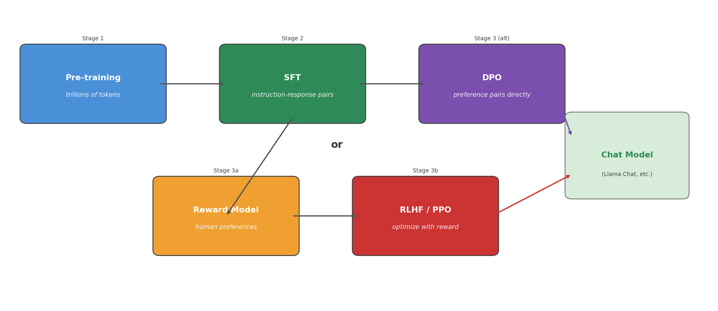
The Full Pipeline
The diagram below shows how all the stages fit together. Pre-training produces a base model that can predict the next token but cannot follow instructions. SFT teaches it to respond to instructions. Then either RLHF (with a reward model and PPO) or DPO aligns the model’s responses with human preferences. The result is the chat model you interact with.
Next Up
This article covered the training side of large language models. How much memory they need, how training is split across GPUs, why training is so expensive, how scaling laws shape model and data choices, why data quality matters, what different layers learn, and how post-training alignment turns a base model into an assistant.
The next step is inference, running the trained model to generate text. In Part 4, I cover how generation works one token at a time, why the KV cache matters, and how decoding strategies like temperature, top-k, and top-p control the style and diversity of the output.