How LLMs Work, Part 1: How LLMs Process Text

How LLMs Work, Part 1: How LLMs Process Text

I have been working as a software engineer building distributed systems for several years, and have been using LLMs extensively in my day-to-day work. But I did not understand how they actually work under the hood. Every time I tried to read something about LLMs, I would get stuck on unfamiliar terminology such as attention, backpropagation, and tokenization, and spend more time on side research than on the actual topic. Over multiple lookups I could follow individual explanations of these terms, but I still could not connect them into a complete understanding of how the system works end to end.

I decided to sit down and read through the fundamentals properly, taking notes so I could refer back to them. The notes kept growing (there was so much I did not know), and eventually turned into this series. My goal was to write the document I wished I had when I started: a first read for any software engineer who wants to understand how LLMs work from the ground up, without needing a background in machine learning or statistics.

The article grew long enough that I have broken it into four parts:

• Part 1 (this post): How LLMs Process Text. Tokenization, embeddings, and the forward pass.
• Part 2: How LLMs Learn: The loss function, backpropagation, and optimizers.
• Part 3: From Toy Model to GPT: Scaling, what the model learns, fine-tuning and RLHF.
• Part 4: Using the Trained Model: Inference, the KV cache, and decoding strategies.

---

What Does Training Mean?

When you type a message into an LLM like Claude, the model generates its response one word (or token) at a time. It reads your message, produces the first word, then reads your message plus the first word it just produced, generates the second word, and so on. Each time, it is answering one question: given everything so far, what should the next token be?

That is the entire objective of training. The model learns to predict the next token.

A model is, at its core, a massive collection of numbers. These numbers are called parameters. Think of them as knobs on a machine: each knob is set to some value, and together all the knobs determine what the machine does. The input text is first converted into numbers too (I will cover how in the Tokenization section below), and then those numbers are multiplied by, added to, and transformed by the model’s parameters at every step. The final output depends entirely on what values the knobs are set to. Llama-3.1-8B has 8 billion parameters.

Before training, most of them are set to small random values. If all parameters started at zero, every part of the model would compute the same output, receive the same gradient, and update identically. The model would be stuck doing the same thing everywhere and could never learn to distinguish different patterns. Random initialization breaks this symmetry, giving each part of the model a different starting point so it can specialize during training. (I cover gradients and how training updates these parameters in Part 2.)

At the start, the model cannot predict anything useful. If you feed it “The cat sat on the” and ask it to predict the next token, it will output something random, maybe “purple” or “seventeen” or a punctuation mark. It has no idea.

Where Do the 8 Billion Parameters Come From?

The parameter count of a model is determined by its architecture choices. For Llama 3.1-8B:

• Vocabulary size: 128,256 tokens
• Embedding dimension: 4,096 (each token is represented as a vector of 4,096 numbers, more on this in the Forward Pass section below)
• Number of layers: 32
• Attention heads: 32 query heads, 8 key/value heads
• Feedforward intermediate size: 14,336

The embedding table alone accounts for 128,256 × 4,096 = ~525 million parameters. Each transformer layer contains attention weight matrices (~42 million parameters) and feedforward weight matrices (~176 million parameters), for roughly 218 million parameters per layer. Multiply by 32 layers and that is ~7 billion. Add the embedding table, the output projection (another ~525 million), and you get roughly 8 billion parameters total.

The parameter count is fixed when you design the architecture. Training does not add or remove parameters. It only changes their values.

Training is the process of adjusting those billions of numbers so the model gets better at predicting what comes next. You show it a sentence like “The cat sat on the mat,” and the model tries to predict each token:

• Given “The”, predict “cat”
• Given “The cat”, predict “sat”
• Given “The cat sat”, predict “on”
• Given “The cat sat on”, predict “the”
• Given “The cat sat on the”, predict “mat”

Each time the model gets it wrong, you measure how wrong it was, and you nudge the parameters in a direction that would have made the prediction a little less wrong. Then you do this again with the next sentence. And the next. And the next. Repeated trillions of times across massive datasets, this helps the model learn patterns which are used to predict the next token. The model never explicitly learns rules like “verbs follow subjects” or “Python uses indentation,” but those patterns end up encoding grammar, facts, reasoning, and style.

The training data is just text: plain text from books, websites, Wikipedia, code repositories, and more. There are no human-written labels saying “the answer here is ‘mat’.” The correct answer is always just the next word in the text. This is called self-supervised learning: the training data provides its own labels, so you do not need anyone to manually annotate anything, which makes it possible to train on trillions of tokens without requiring a human labeler.

---

The Training Data

What the Data Looks Like

LLMs train on text. A lot of text. The training data for a modern LLM is a mix of web pages, books, scientific papers, code, forum posts, and more. Here are some of the publicly known datasets:

• Common Crawl: a nonprofit organization that crawls the web and makes the data publicly available. It has been running since 2008 and has accumulated petabytes of raw HTML. Most LLM training datasets start with Common Crawl and then filter and clean it heavily.
• The Pile: an 825 GB curated dataset created by EleutherAI (Gao et al. 2021). It combines 22 different sources including PubMed abstracts, ArXiv papers, GitHub code, StackExchange posts, Wikipedia, Project Gutenberg books, and more. The Pile was designed to be diverse, covering many domains so the model does not just learn internet-speak.
• RedPajama: an open reproduction of the LLaMA training dataset, created by Together AI in 2023. It contains 1.2 trillion tokens sourced from Common Crawl, Wikipedia, GitHub, books, ArXiv, and StackExchange.

For proprietary models like GPT-4, the exact training data is not public. OpenAI has described it as a mix of publicly available data and data licensed from providers, but the specifics are not disclosed.

The raw data is not clean. It contains duplicates, low-quality text, spam, toxic content, and personally identifiable information. A large part of the training pipeline is data cleaning and filtering: removing duplicates, filtering out low-quality pages, stripping personal information, and balancing the mix of different sources. The quality of the training data has a direct impact on the quality of the model. As the famous saying in data science goes: garbage in, garbage out.

Tokenization: From Text to Numbers

The model cannot read text. It works with numbers. Tokenization is the process of converting text into a sequence of integer IDs that the model can process.

The simplest approach would be to split text by spaces and assign each word a number. “The” gets ID 1, “cat” gets ID 2, and so on. The problem is that this creates a huge vocabulary. English alone has hundreds of thousands of words, and when you add technical terms, names, misspellings, and words from other languages, the vocabulary explodes. A word the model has never seen before would have no ID at all.

Another approach is character-level tokenization: treat each character as a token. The vocabulary is tiny (a few hundred entries covering letters, digits, and punctuation), but sequences become very long. The word “understanding” becomes 13 tokens instead of 1 or 2, and the model has to learn how to spell every word from scratch.

The middle ground that modern LLMs use is subword tokenization. The most common method is Byte Pair Encoding (BPE), originally a data compression algorithm by Philip Gage in 1994, adapted for machine translation by Sennrich et al. 2016 and now used by GPT, Llama, and most modern LLMs.

BPE works like this:

1. Start with individual bytes as the initial vocabulary. Every piece of text on a computer is stored as a sequence of bytes. A byte is 8 bits, which means it can represent 2^8 = 256 distinct values (0 to 255). Simple ASCII characters like a, Z, or . each map to a single byte. Characters from other languages or scripts take multiple bytes in UTF-8 encoding: the Chinese character 猫 is three bytes, and an emoji like 🐱 is four bytes. These 256 possible byte values become the starting vocabulary. Starting from bytes instead of alphabet characters means the tokenizer can handle any text in any language, because everything is bytes at the bottom. GPT-2, Llama, and most other large language models use BPE-based tokenizers. The exact implementations differ between models, but the core algorithm is the same. The tokenizer is built once, before model training starts, by running BPE on the full training dataset (or a large representative sample of it). Once the vocabulary is fixed, it does not change during training.
2. Scan the training text and count every pair of adjacent tokens.
3. Find the most frequent pair. Merge it into a single new token. Add it to the vocabulary. The original tokens are not removed: for example, if t and h merge into th, both t and h remain in the vocabulary because other words might still need them individually. The vocabulary only grows.
4. Repeat until the vocabulary reaches the desired size.

Here is a small example. Suppose our training text is: “low lower lowest low lower”

For simplicity, this example uses only ASCII characters, so each character is one byte. The starting tokens are: l, o, w, ` , e, r, s, t`

Count adjacent pairs:

• l + o appears 5 times (in each “low”)
• o + w appears 5 times
• w + ` ` appears 2 times
• and so on

The most frequent pairs are l + o and o + w, both appearing 5 times. BPE picks one (implementations break ties differently, here we take l + o first). Merge it into a new token lo. Now our text in tokens is: lo, w, ` , lo, w, e, r, , lo, w, e, s, t, , lo, w, , lo, w, e, r`.

Next most frequent: lo + w (5 times). Merge into low. Now: low, ` , low, e, r, , low, e, s, t, , low, , low, e, r`.

Next most frequent: low + e (3 times). Merge into lowe. And so on.

After enough merges, common words become single tokens and rare words get split into pieces. The word “understanding” might become two tokens: “under” + “standing”. The word “unrelated” might become “un” + “related”. Very rare words get split into more pieces, all the way down to individual characters if needed.

The vocabulary size is a design choice, and it directly controls how many merges BPE performs. The algorithm starts with 256 base tokens (the byte values). Each merge adds exactly one new token, so the number of merges is roughly: target vocabulary size minus 256 (real tokenizers may also include special tokens and reserved entries, but the principle is the same). If you set the target to 32,000, BPE performs 32,000 - 256 = 31,744 merges and then stops. If you set it to 128,256, it performs 128,256 - 256 = 128,000 merges before stopping.

To see this concretely, lets go back to our “low lower lowest” example. We started with 8 character tokens. If we set the target vocabulary size to 10, BPE can only do 2 merges: it creates lo and then low, and stops. The word “lower” is still three tokens: low, e, r. But if we set the target to 12, BPE gets 4 merges: it goes further and merges low + e → lowe, then lowe + r → lower. Now “lower” is a single token. A larger vocabulary gave the algorithm room for more merges, and those extra merges collapsed a three-token word into one.

GPT-2 uses 50,257 tokens. Llama 2 uses 32,000 tokens. Llama 3 uses 128,256 tokens. With Llama 2’s smaller vocabulary, a word like “understanding” might be split into two tokens: “under” + “standing.” With Llama 3’s larger vocabulary, BPE had room for far more merges, so “understanding” ends up as a single token. This makes sequences shorter. The model processes and generates one token per step, so fewer tokens means fewer steps to produce the same text, which means faster generation. The tradeoff is size. The model needs an embedding table that converts each token ID into a vector of numbers the model can work with (I cover this in the Forward Pass section below). Each token gets its own row in this table, so 128,256 tokens means 128,256 rows. At the other end, the model needs to produce a score for every possible next token which I’ll cover in the Forward Pass section. So larger vocabulary means larger embedding table and larger output layer, both of which take more memory.

After BPE finishes, the result is a fixed vocabulary where each token is assigned an integer ID based on its position in the list. Tokenizing a sentence means splitting it into tokens using the learned merge rules, then replacing each token with its ID. So “The cat sat on the mat” might become [464, 3797, 3290, 319, 278, 15021]. These are the numbers the model actually works with.

Scale: How Much Data

To get a sense of the scale:

• GPT-3 trained on roughly 300 billion tokens (Brown et al. 2020).
• Llama 2 trained on 2 trillion tokens (Touvron et al. 2023).
• Llama 3 trained on over 15 trillion tokens (Meta, 2024).

To put 2 trillion tokens in perspective: if the average book has about 80,000 words (roughly 100,000 tokens), then 2 trillion tokens is about 20 million books. The Library of Congress has about 41 million books and is the largest library in the world by catalogue size. Llama 2 trained on roughly half as many books as the largest library in the world.

You might assume that more data always means a better model, but it is not that simple. For a fixed compute budget, there is an optimal ratio between model size and training data. Train a model with many parameters (meaning more capacity to learn complex patterns) on too little data and it underfits: the model has room to learn but has not seen enough examples, so it makes poor predictions. Train a small model on too much data and you waste compute on a model that does not have enough parameters to absorb what it is being shown. I cover the math behind this tradeoff in the Chinchilla scaling laws section in Part 3.

---

The Forward Pass: From Tokens to Prediction

A Brief Recap of the Architecture

I covered embeddings, attention mechanisms, and weight matrices in detail in my TurboQuant post. Here is the quick version.

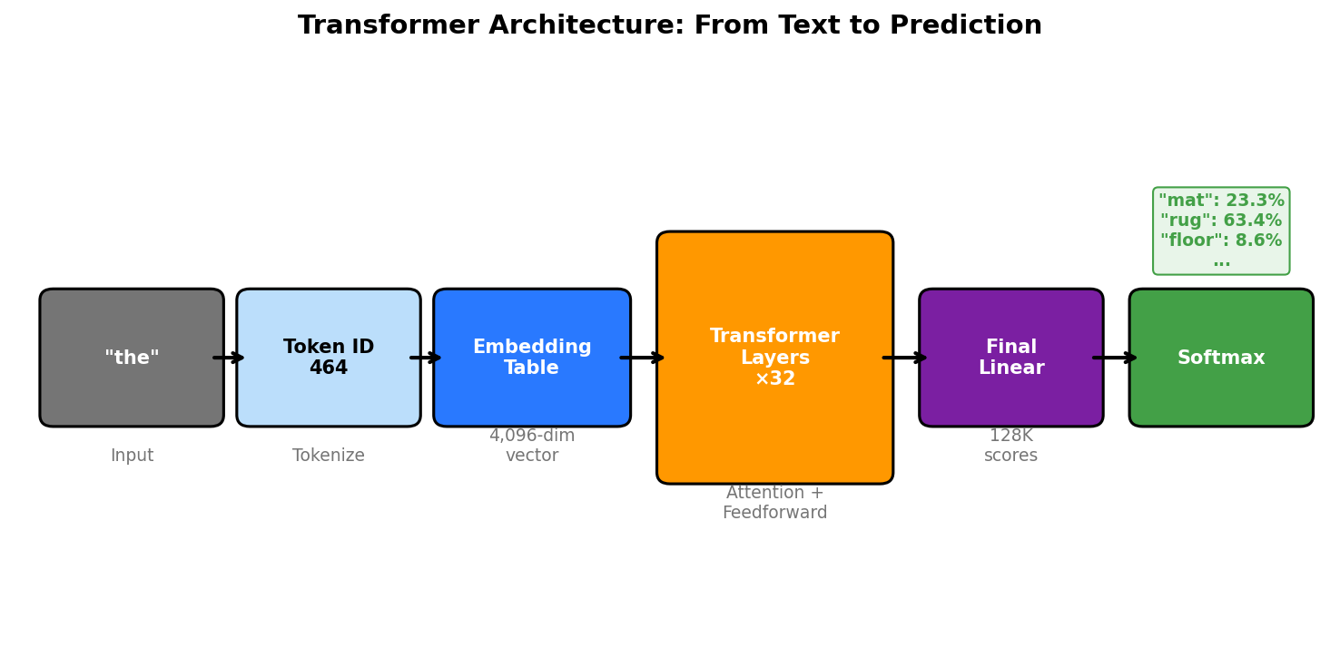
You start with a token ID, which is just a number. The model looks up that ID in the embedding table (introduced in the Tokenization section above). The table has one row per token in the vocabulary. Each row is a list of numbers. The length of this list is called the embedding dimension. For Llama-3.1-8B, the embedding dimension is 4,096, meaning each token is represented by 4,096 numbers. A larger embedding dimension gives each token more room to encode nuanced information (more “slots” to represent different aspects of meaning), but it also increases the parameter count and computation throughout the model, since every layer operates on vectors of this size. Smaller models like GPT-2 Small use 768 dimensions. Llama 3.1-70B uses 8,192. Once the vocabulary is fixed (from the tokenization step above), the model creates the embedding table with one row per token. Before training, these rows are filled with small random numbers. They carry no meaning yet. During training, they get adjusted so that tokens used in similar contexts end up with similar numbers. To see why, consider how training works. The model uses the embedding vector to predict the next token. When it gets the prediction wrong, it adjusts the vector to make the prediction better. Now think about “dog” and “cat.” Both appear in sentences like “The __ sat on the mat” and “She fed the __.” The correct prediction after each word is the same. So the training process applies similar adjustments to both vectors: any vector that helps predict a noun in the object position gets tweaked in the same direction. After many training steps, the embeddings for “dog” and “cat” end up close to each other in the 4,096-dimensional space. More generally, embeddings encode something like “semantic similarity”: words used in similar contexts get similar vectors.

To make this concrete, consider the word “apple.” The embedding table has exactly one row for the token “apple.” Every time “apple” appears in any sentence, the model starts with the same 4,096-dimensional vector, one that has been shaped by all the training data the model has seen so far. There is no separate “apple the fruit” and “apple the company” in the table.

During training, both meanings compete for the same row. When the model trains on “I ate an apple for lunch,” backpropagation nudges the “apple” embedding toward values that help predict food-related words. When it trains on “Apple announced a new iPhone,” the same row gets nudged toward tech-related values. Over billions of such updates, the embedding settles on a compromise: the 4,096 numbers encode something like “a common English noun that appears in food contexts and technology contexts.” It captures what is shared across all uses of “apple” but cannot fully represent any single meaning.

This is fine because the embedding does not need to do all the work. It is a starting point. Once the vector enters the transformer layers, the attention mechanism looks at the surrounding words (“ate” and “lunch” vs “announced” and “iPhone”) and transforms the generic “apple” vector into something context-specific. By the time it passes through all 32 layers, the two instances carry completely different representations: one encoding “edible fruit” and the other encoding “technology company.”

In practice, the model does not process one sentence at a time. The training data is split into fixed-length sequences (4,096 tokens for Llama 2) and grouped into batches. A single batch for Llama 2 contains 1,024 sequences of 4,096 tokens each, roughly 4 million tokens total. That is maybe a few chapters from different books, all processed in parallel. For clarity, I will walk through the forward pass using a single short example: “The cat sat on the.”

This vector then flows through a stack of transformer layers. Each layer has two main components: an attention mechanism and a feedforward network.

Attention

Attention is about relationships between tokens. It mixes information across the sequence.

Attention works through three vectors that are computed for each token: a query, a key, and a value.

• The query is what a token is looking for. Think of it as a question: “what kind of context do I need?”
• The key is what a token advertises about itself. Think of it as a label: “here is what I contain.”
• The value is the actual information the token carries. If the query and key match well, this is what gets passed along.

The attention score between two tokens is the dot product of one token’s query and the other token’s key. A high dot product means “these two tokens are relevant to each other.” The scores get normalized (using softmax), and then each token’s output is a weighted sum of all the value vectors, where the weights are the attention scores.

A concrete example: in “The cat sat on the,” when computing attention for the second “the”:

"the" produces a query:   "I need context about what kind of thing follows"
"sat" has a key:           "I am a verb describing a sitting action"
"on"  has a key:           "I am a preposition indicating location"

query("the") · key("sat") = high score   → "sat" is relevant
query("the") · key("on")  = high score   → "on" is relevant
query("the") · key("The") = low score    → the first "The" is less relevant

Output for "the" = 0.4 × value("sat") + 0.35 × value("on") + 0.15 × value("cat") + 0.1 × value("The")

When the model is processing the word “the” (the second “the”) in “The cat sat on the,” it needs to know what came before. The attention mechanism lets the current token look back at all previous tokens and decide which ones matter. For this “the,” the model might learn to pay attention to “sat” and “on” because they signal that a location or surface noun is coming next. Attention does this for every token in the sequence simultaneously: each token’s vector gets updated to carry information from the tokens it attended to. After attention, the vector for “the” is no longer just about the generic word “the.” It now encodes something like “‘the’ in the context of something that sat on something,” which is useful for predicting what comes next.

An important detail is within a single layer, all tokens are processed simultaneously. When computing attention for “sat,” it uses the original embedding of “cat,” not an attention-updated version of “cat” from the same layer. All tokens go through the same attention step at the same time using matrix multiplication, which is a major reason transformers are fast to train. The refinement happens across layers: layer 2’s attention uses the outputs of layer 1 (which have already been through attention and feedforward), so “sat” in layer 2 attends to an already-refined version of “cat.” This is how stacking 32 layers helps as each layer builds on richer representations from the layer below.

Positional Encoding: RoPE

The attention mechanism described above lets each token see the tokens that came before it, but it does not know their order. It sees a set of vectors and computes dot products against them. If “cat” and “sat” swapped positions, the attention scores would not change because attention operates on content, not position. Without position information, “the cat sat on the mat” and “the sat cat on mat the” would look the same to the model. Word order carries meaning (“the dog bit the man” vs “the man bit the dog”), so the model needs a way to encode position.

The original Transformer paper (Vaswani et al. 2017) solved this by adding position information directly to each token’s embedding. Each position in the sequence gets a unique pattern of numbers, computed from a fixed formula. Position 0 always gets the same pattern, position 1 always gets the same pattern, and so on. The model does not learn these patterns. They are hardcoded. This way, even if two tokens have the same embedding, the model can tell them apart by their position.

Modern LLMs like Llama use Rotary Position Embeddings (RoPE). Instead of adding a position vector, RoPE rotates the query and key vectors by an angle that depends on their position. Think of it geometrically: tokens at similar positions get rotated by similar amounts, so their dot products (which determine attention weights) remain high. Tokens far apart get very different rotations, which changes their dot products. The model can learn how position affects meaning because the rotation encodes relative distance directly into the attention computation.

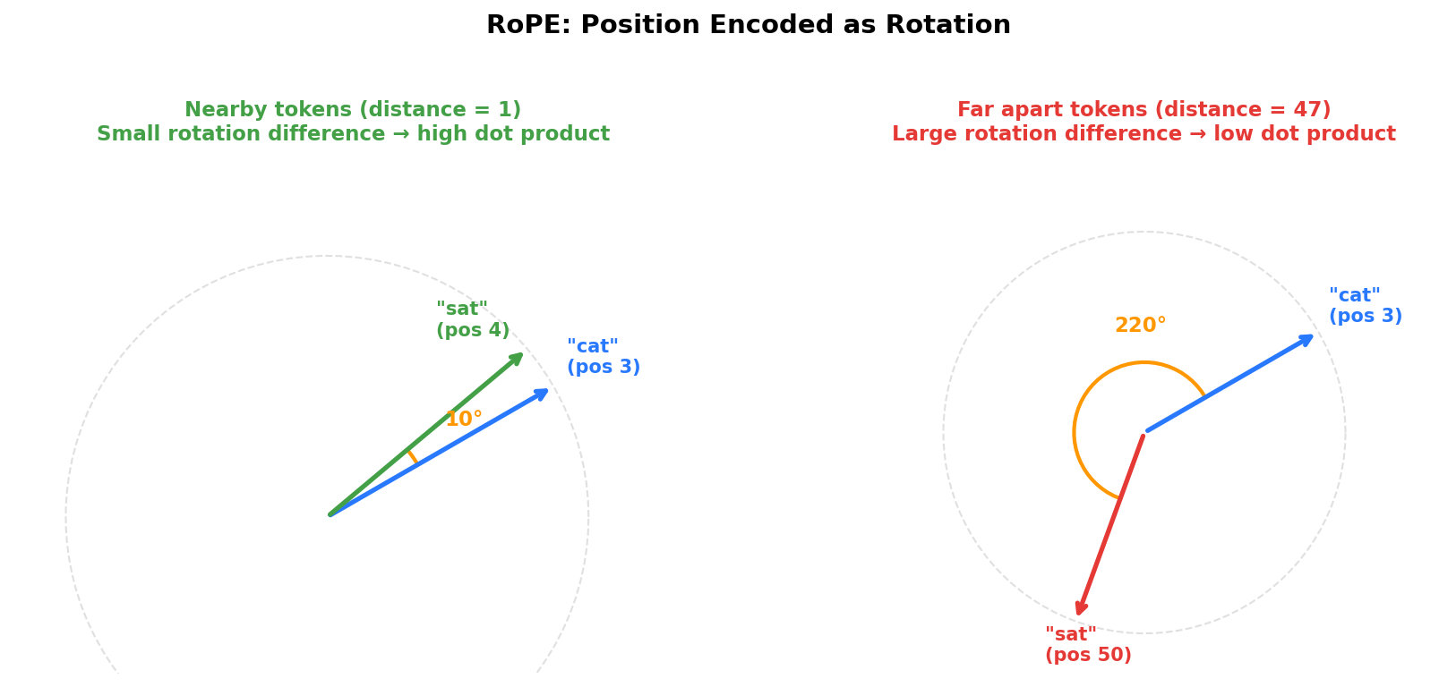
The original Transformer paper was encoding the absolute position in the sentence, whereas RoPE encodes relative position. The attention score between two tokens depends on the distance between them, not where they sit in the sequence. “The cat” means the same thing whether it appears at position 0 or position 500.

Multi-Head Attention

The attention mechanism described above computes one set of attention weights. But a single attention pass can only capture one type of relationship at a time. In the sentence “The cat sat on the mat,” there are multiple things worth paying attention to simultaneously: “cat” is the subject of “sat,” “on” connects to “mat,” “the” modifies “mat.” A single set of attention weights has to pick one pattern to focus on, or blend them together into a compromise.

Transformers solve this by running multiple attention computations in parallel, called heads. Each head has its own learned weights and can focus on a different relationship.

Concretely, in the sentence “The cat sat on the mat,” one attention head might focus on subject-verb relationships (“cat” → “sat”), another on prepositional phrases (“on” → “mat”), and another on determiner-noun pairings (“the” → “cat”). All three computations happen at the same time, then the results get combined. This gives the model multiple perspectives on what matters at each step.

Llama 3 8B has 32 attention heads. The 4,096-dimensional embedding vector gets split into 32 chunks of 128 dimensions each. Each head runs attention independently on its 128-dimensional chunk. After all heads are done, the results are concatenated back into a 4,096-dimensional vector. Each head can learn to focus on different relationships in the input. One head might attend to syntactic structure, another to semantic similarity, another to positional proximity. This representational diversity is the main reason for using multiple heads. This is why it is called “multi-head” attention: 32 different “perspectives” on the same input, each attending to different parts of the sequence.

Llama 3 also uses a technique called Grouped Query Attention (GQA). In standard multi-head attention, the model computes 32 different key vectors and 32 different value vectors for each token, one per head. Each key is a different description of what the token contains, tailored for one specific query head. Head #0 might describe the token “sat” as “action verb,” while head #5 describes the same “sat” as “past tense word,” and head #12 describes it as “word near the middle of the sentence.”

In GQA, the model only computes 8 key vectors and 8 value vectors per token. Query heads #0, #1, #2, #3 all use the same key and value vectors (computed by key/value head #0) when attending to any token. So when all four of them look at the token “sat,” they see the same description of it, but each query head can still produce different attention scores because their queries are different. The keys just need to provide a good enough description for the queries to match against. Eight different descriptions per token turns out to be enough for 32 different queries to find what they need. GQA trades a small amount of model quality for a 4x reduction in KV cache memory. For inference-heavy workloads serving millions of users, that memory saving matters enormously. I cover the KV cache in detail in Part 4. The smaller Llama 2 models (7B and 13B) used the standard approach with 32 separate key/value heads. The Llama 2 70B model used GQA.

Feedforward Network

After attention, each token’s vector carries blended information from the tokens it attended to. But attention can only mix existing information. It takes a weighted average of the vectors it attended to. Going back to the example, when processing “the” in “The cat sat on the,” attention blends signals from “sat” and “on” into the vector for “the.” If “sat” carries a feature for “action verb” and “on” carries a feature for “preposition,” the output might be something like “0.4 × action verb + 0.35 × preposition.” That is useful context, but it is still a combination of existing features. It cannot create a new feature like “expecting a surface noun” that neither “sat” nor “on” had on their own.

The feedforward network creates those new features. It takes each token’s post-attention vector independently (it does not look at other tokens) and runs it through two matrix multiplications with an activation function in between.

The activation function is critical here. Without it, stacking two matrix multiplications would be pointless: multiplying by matrix A and then by matrix B is mathematically the same as multiplying by one combined matrix AB. No matter how many layers you stack, the result collapses to a single linear transformation, which can only learn straight-line relationships.

The activation function breaks this by introducing nonlinearity. A simplified example is ReLU (Rectified Linear Unit), which says: if the number is positive, keep it; if it is negative, replace it with zero. (Modern LLMs like Llama use more sophisticated gated variants like SwiGLU, but the principle is the same: introduce nonlinearity.) With this nonlinear step between the two matrix multiplications, the feedforward network can learn transformations that a single matrix multiplication never could. It can take “0.4 × action verb + 0.35 × preposition” and produce a new feature like “expecting a surface noun.”

The first matrix multiplication expands the vector from 4,096 dimensions to 14,336 (for Llama 3 8B; sizes vary by model). The second shrinks it back to 4,096. The expansion gives the network room to compute many intermediate features before compressing back down.

To put this in perspective, the feedforward network is where most of the model’s parameters live. For Llama 3 8B, each layer’s feedforward network has roughly 176 million parameters, compared to about 42 million for the attention mechanism. Across 32 layers, that is about 5.6 billion parameters in the feedforward networks alone, out of 8 billion total. This is where the bulk of the model’s “knowledge” is stored.

Researchers have found that individual components within the feedforward network often correspond to specific, interpretable concepts (Geva et al., 2021). One might activate when the input is about sports, another when processing Python code, another when it sees the name of a city. The network discovers these patterns during training as a byproduct of learning to predict the next token, and organizes them across its 14,336 intermediate dimensions.

One way to think about the division of labor between attention and the feedforward network is that attention gathers evidence. It looks at the surrounding tokens and collects relevant context. The feedforward network draws conclusions from that evidence. Attention gathers that “sat” and “on” are nearby, and the feedforward network figures out that this combination means a surface noun is likely coming next.

So after one layer of attention followed by one feedforward network, the vector for “the” has gone from meaning just “the word ‘the’” to something closer to “a determiner preceding a noun that is the object of ‘sat on.’”

Llama-3.1-8B stacks 32 of these layers on top of each other. The output of layer 1 feeds into layer 2, which feeds into layer 3, and so on. Each layer refines the representation further: early layers tend to pick up basic patterns like grammar and word relationships, while later layers encode more abstract things like meaning and context.

After all 32 layers, you have a final vector of 4,096 numbers for each token in the input. For “The cat sat on the,” that means 5 vectors, each 4,096 numbers long.

These 5 vectors are not stored anywhere permanently. They are temporary working copies, computed fresh every time the model processes a sentence. The embedding table still has just one row for “the.” When the model starts processing this sentence, it pulls two copies of that same row (one for each “the” in the input). Both copies start identical. But as they flow through the 32 layers, attention modifies each copy based on its surrounding context. The first “The” at position 0 had no prior tokens to attend to. The second “the” at position 4 has access to “cat,” “sat,” “on” and can ground itself with more context. By the time they exit layer 32, the two copies carry very different vectors.

This is the same idea as the “apple” example from earlier. The embedding table always has one row for “apple,” one row for “the,” one row for every token. That row is a generic starting point. The transformer layers create context-specific representations during each forward pass, but those representations are temporary. They are used to predict the next token and then discarded. The embedding table row itself only gets adjusted during training as part of the parameter update process (covered in Part 2).

During training, the model processes a sentence, produces temporary vectors, uses them to predict the next token, and compares that prediction to the actual next token in the training text. The difference between the prediction and reality is used to adjust the permanent parameters slightly. This repeats trillions of times. Over those trillions of updates, the parameters get shaped so that the model becomes good at transforming generic token embeddings into context-rich representations. I cover the mechanics of how this adjustment works in Part 2.

During inference, the parameters are fixed. The model still creates temporary copies and transforms them through the layers, just like during training, but there is no adjustment step. The parameters have already been shaped by training to produce useful transformations.

The Final Layer: Predicting the Next Token

At this point, the model has processed “The cat sat on the” through 32 layers and produced a 4,096-number vector for each token. To predict the next token, the model only needs the vector for the last token (“the”), because that vector has already absorbed context from all previous tokens through attention.

Now the model needs to answer: out of every token in the vocabulary, which one should come next? For Llama 3, that means choosing from 128,256 possible tokens. The model needs to produce a score for every single one.

It does this with one matrix multiplication. The 4,096-number vector gets multiplied by a large matrix with 4,096 rows and 128,256 columns. Each column in this matrix corresponds to one token in the vocabulary. The multiplication produces a dot product between the vector and each column, giving a single number per token. The result is a vector of 128,256 numbers, one score per possible next token.

These raw scores are called logits. A logit is just a number that says how strongly the model favors a particular token. For our example, the logits might look something like:

"mat"    → 2.0
"floor"  → 1.0
"table"  → 0.1
"sky"    → -1.0
"rug"    → 3.0
... (128,251 other tokens with their own scores)

The model thinks “rug” is most likely (highest score at 3.0), followed by “mat” at 2.0, then “floor” at 1.0. But logits are not probabilities. They can be negative, they can be very large, and they do not add up to 1. They are just raw scores. To turn them into probabilities, the model uses softmax.

Softmax: Turning Numbers into Probabilities

To convert logits into actual probabilities, the model applies a function called softmax. Softmax does two things at once. First, it takes the exponential of each logit, which makes all values positive. Second, it divides each value by the sum of all exponentials, which normalizes everything so the probabilities add up to 1.

The formula:

softmax(z_i) = e^(z_i) / sum(e^(z_j) for all j)

Here is a concrete example. Suppose the model outputs logits [2.0, 1.0, 0.1, -1.0, 3.0] for five possible next tokens: “mat”, “floor”, “table”, “sky”, and “rug”.

Step 1: Compute e^z for each logit.

e^2.0  = 7.39
e^1.0  = 2.72
e^0.1  = 1.11
e^-1.0 = 0.37
e^3.0  = 20.09

Step 2: Add them all up.

7.39 + 2.72 + 1.11 + 0.37 + 20.09 = 31.67

Step 3: Divide each exponential by the sum.

7.39  / 31.67 = 0.233
2.72  / 31.67 = 0.086
1.11  / 31.67 = 0.035
0.37  / 31.67 = 0.012
20.09 / 31.67 = 0.634

The probabilities are now [0.233, 0.086, 0.035, 0.012, 0.634]. The model thinks “rug” is most likely with 63.4% probability, followed by “mat” at 23.3%, then “floor” at 8.6%, and so on. All probabilities are positive and they add up to 1.

One thing to note: softmax amplifies differences between logits. The token with the highest logit gets a disproportionately large share of the probability mass. The difference between 3.0 and 2.0 was only 1 point in logit space, but in probability space, “rug” got 63.4% while “mat” got only 23.3%. This happens because the exponential function grows very fast.

Temperature: Controlling Randomness

When you use an LLM through an API or a playground, there is a parameter called temperature that controls how random the output is. Temperature works by scaling the logits before softmax is applied. You divide all logits by the temperature value, then softmax proceeds as normal.

• temperature = 1.0: no scaling, softmax behaves normally.
• temperature = 0.5: divide logits by 0.5 (same as multiplying by 2). The logits become more extreme. Softmax produces a sharper distribution. The top token dominates even more. Output becomes more predictable and repetitive.
• temperature = 2.0: divide logits by 2.0, making them smaller. Softmax produces a flatter distribution. More tokens get reasonable probabilities. Output becomes more creative but also more likely to be incoherent.

Using the same example, starting logits are [2.0, 1.0, 0.1, -1.0, 3.0].

With temperature = 0.5, divide by 0.5: [4.0, 2.0, 0.2, -2.0, 6.0]

e^4.0  = 54.60       54.60  / 466.78 = 0.117
e^2.0  = 7.39         7.39  / 466.78 = 0.016
e^0.2  = 1.22         1.22  / 466.78 = 0.003
e^-2.0 = 0.14         0.14  / 466.78 = 0.0003
e^6.0  = 403.43     403.43  / 466.78 = 0.864

“rug” now gets 86.4% instead of 63.4%. The distribution is much sharper.

With temperature = 2.0, divide by 2.0: [1.0, 0.5, 0.05, -0.5, 1.5]

e^1.0   = 2.72       2.72 / 10.51 = 0.259
e^0.5   = 1.65       1.65 / 10.51 = 0.157
e^0.05  = 1.05       1.05 / 10.51 = 0.100
e^-0.5  = 0.61       0.61 / 10.51 = 0.058
e^1.5   = 4.48       4.48 / 10.51 = 0.426

Now “rug” gets only 42.7% instead of 63.4%, and other tokens have more reasonable chances. “table” jumped from 3.5% to 10.0%. The distribution is flatter.

Token	Logit	temp=1.0	temp=0.5	temp=2.0
mat	2.0	23.3%	11.7%	25.9%
floor	1.0	8.6%	1.6%	15.7%
table	0.1	3.5%	0.3%	10.0%
sky	-1.0	1.2%	0.03%	5.8%
rug	3.0	63.4%	86.4%	42.7%

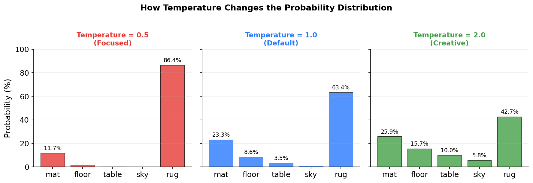
That is why low temperature gives you predictable, focused output, and high temperature gives you creative, surprising output.

Context Window

Earlier I mentioned that the training data is split into fixed-length sequences of 4,096 tokens. This length is the model’s context window, the maximum number of tokens it can process at once. Llama 2 was trained on sequences of 4,096 tokens, so during inference it can handle up to 4,096 tokens of context. Llama 3.1 extended the context window to 128,000 tokens by doing additional training on longer sequences and adjusting the RoPE scaling to handle positions it had not seen before.

The context window has a direct impact on attention cost. Attention computes a score between every pair of tokens, which means n tokens require n² scores per attention head per layer. Doubling the context length quadruples the computation.

Memory also scales with context length. During inference, the model stores the key and value vectors for every token it has seen so far (this is the KV cache, covered in Part 4). Longer contexts mean more stored vectors and more GPU memory. A 4,096-token context is roughly 3,000 words. A 128,000-token context is roughly 100,000 words.

For developers building on top of LLMs, the context window determines how much text the model can “see” at once. If your prompt plus the model’s response exceeds the context window, the oldest tokens fall off. The model can no longer see them. This is why long conversations sometimes lose coherence or forget details from earlier in the chat.

---

What Happens Next

In this article I covered how LLMs process text: tokenization converts text into numbers, those numbers are represented as embeddings (vectors of 4,096 numbers), and the transformer layers refine these embeddings by mixing information across the sequence through attention and creating new features through the feedforward network. After 32 layers, the final layer produces a probability distribution over the entire vocabulary for the next token.

All of this assumes the model has been trained. Before training, the parameters are random and the predictions are useless. The model needs a way to measure how wrong its predictions are, compare them to the actual text, and adjust its parameters to do better next time. That is what I will cover in the next article Part 2: How LLMs Learn. We will go over the loss function, backpropagation, and the optimizers which drive the learning process.

---

Sources

Vaswani et al., 2017. Attention Is All You Need

Sennrich et al., 2016. Neural Machine Translation of Rare Words with Subword Units

Brown et al., 2020. Language Models are Few-Shot Learners (GPT-3)

Touvron et al., 2023. Llama 2: Open Foundation and Fine-Tuned Chat Models

Meta, 2024. Llama 3 Model Card

Gao et al., 2021. The Pile: An 800GB Dataset of Diverse Text for Language Modeling

Su et al., 2021. RoFormer: Enhanced Transformer with Rotary Position Embedding

---

<

Previous Post

Java Virtual Threads: The Pinning Problem, the Deadlock, and the Fix in Java 24

>

Blog Archive

Archive of all previous blog posts