How LLMs Work, Part 2: How LLMs Learn

How LLMs Work, Part 2: How LLMs Learn

In Part 1, I covered tokenization and the forward pass: how text becomes numbers, and how those numbers flow through a transformer to produce predictions. But a model with random parameters makes random predictions. It needs to learn.

In this article, we will explore the loss function that measures how wrong the model is, backpropagation that computes gradients, and the optimizers (SGD, Adam) that adjust billions of parameters. I go through gradient descent and learning rate schedules with worked examples, and finish with a complete training loop you can run yourself.

---

The Loss Function: Measuring How Wrong the Model Is

Let’s go back to the training sentence from earlier: “The cat sat on the mat.” The model just predicted probabilities for each possible next token after “The cat sat on the.” The actual next word in the training data is “mat,” but the model assigned “mat” a probability of only 0.233 (23.3%) and gave “rug” 63.4%. The model got it wrong. We need a way to measure how wrong it was. That measurement is called the loss.

The loss function used by virtually all language models is cross-entropy loss. The formula is as follows:

loss = -log(probability of the correct token)

Here log is the natural logarithm (base e). Computing the loss for our example: The correct token is “mat”, and the model gave it probability 0.233.

loss = -log(0.233) = -(-1.457) = 1.457

What if the model had been more confident and correct? If it gave “mat” probability 0.95:

loss = -log(0.95) = 0.051

That gives a loss of 0.051, compared to 1.457 when the model assigned only 23.3% to “mat.” The model is being rewarded for being confident in the right answer.

What if the model had been very wrong? If it gave “mat” probability 0.01:

loss = -log(0.01) = 4.605

Very high. The loss function heavily penalizes confident wrong predictions.

Here is a table showing how loss changes with the model’s confidence in the correct answer:

Probability of correct token	Loss
0.01	4.605
0.10	2.303
0.25	1.386
0.50	0.693
0.75	0.288
0.95	0.051
0.99	0.010

As the pattern shows, loss is 0 when the model assigns probability 1.0 to the correct token. As the probability of the correct token drops toward 0, the loss climbs toward infinity. The loss function is small when the model gives the correct token a high probability, but if the model gives the correct token a very low probability (meaning it was very wrong), the loss is very large.

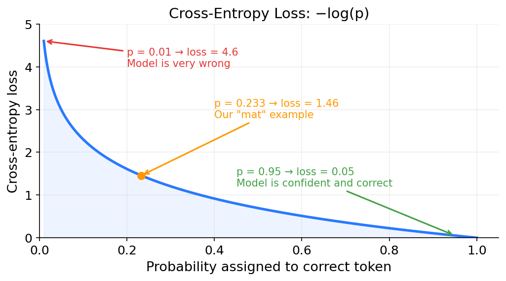
The goal of training is to minimize the average loss across all tokens in the training data. If we have a dataset with one million tokens, we compute the loss for each token’s prediction, add them all up, and divide by one million. We want that average number to be as small as possible.

There is one more metric you will see in LLM papers: perplexity. It is defined as:

perplexity = e^(average loss)

If the average cross-entropy loss across all tokens in a dataset is 2.5, then perplexity = e^2.5 = 12.18. Intuitively, perplexity measures how many tokens the model is “confused between” on average. A perplexity of 12 means the model is, on average, as uncertain as if it were choosing randomly between 12 equally likely tokens. Lower perplexity means a better model. Researchers report both because they are two ways of looking at the same thing: loss is what the optimizer actually minimizes (it is the raw number the math works with), and perplexity gives a more human-interpretable scale. “The model is confused between 12 tokens on average” is easier to reason about than “the loss is 2.5.”

---

Backpropagation: How the Model Learns from Mistakes

We now have a number (the loss) that tells us how wrong the model is. The question is: how do we adjust the model’s parameters to make the loss smaller?

There are billions of parameters. We cannot just try random changes and hope for the best. We need a systematic way to figure out which direction to adjust each parameter.

Gradients: Which Way Is Downhill?

Imagine you are standing on a hilly landscape and you want to get to the lowest point. You are blindfolded, so you cannot see the whole landscape. But you can feel the slope of the ground under your feet. If the ground slopes downward to your left, you step left. If it slopes downward in front of you, you step forward. Each step takes you a little lower.

A gradient is the mathematical version of “the slope under your feet.” For each parameter in the model, the gradient tells you: if I increase this parameter by a tiny amount, does the loss go up or down, and by how much?

Concretely: suppose one of the 8 billion parameters in the model is a number w = 0.5. The loss right now is 1.457 (from our “mat” example). We want to know: if we change w by a tiny amount, does the loss go up or down? We cannot just try every possible change because there are 8 billion parameters. Instead, we compute the gradient using calculus (the chain rule, covered in the next section). The gradient is a single number that tells us the answer. Suppose the gradient of the loss with respect to w comes out to +0.3. The sign tells us the direction: positive means increasing w makes the loss worse, negative means increasing w makes the loss better. The magnitude tells us how sensitive the loss is to this parameter. To see what +0.3 means concretely, imagine nudging w upward by a tiny amount, say 0.001. The gradient says the loss would change by approximately gradient × nudge = 0.3 × 0.001 = 0.0003. Since the gradient is positive, the loss goes up by 0.0003. That is bad, because we want the loss to go down. So we should nudge w in the other direction, downward.

That is the entire idea:

• Positive gradient means increasing this parameter makes the loss worse. Decrease it.
• Negative gradient means increasing this parameter makes the loss better. Increase it.
• Large gradient means this parameter has a big effect on the loss right now.
• Gradient near zero means this parameter barely matters for this particular prediction.

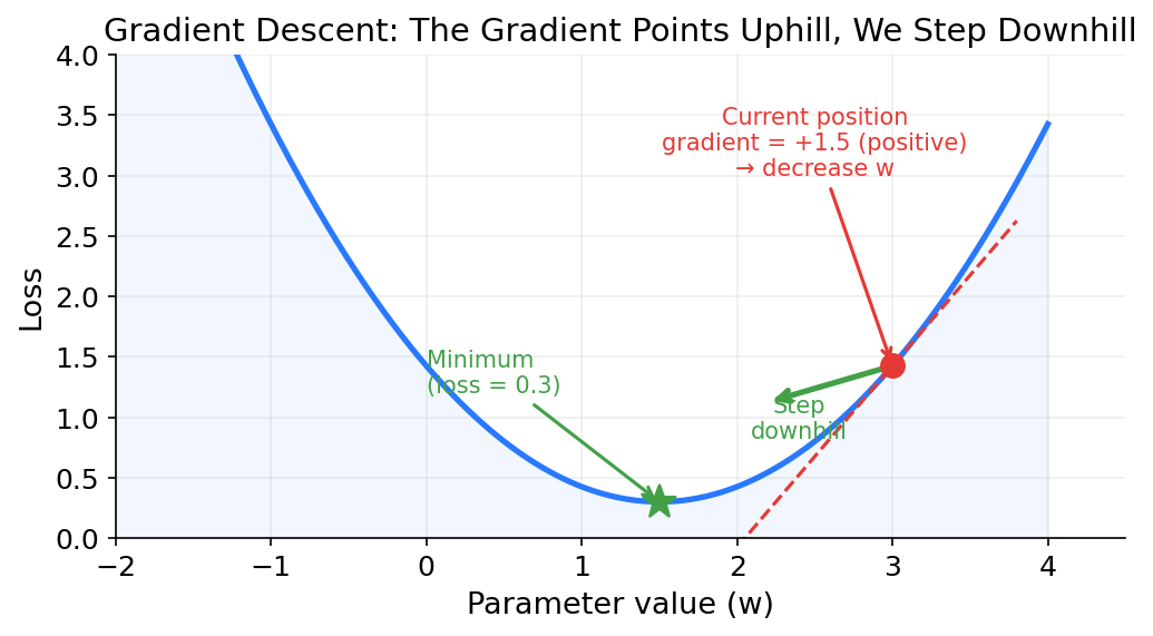
To visualize how gradients work, imagine a model with just one parameter w. In reality there are 8 billion parameters, but we can only draw a 2D chart, so we simplify down to one. The x-axis is the value of that parameter. The y-axis is the loss the model would produce if the parameter had that value (with all other parameters held fixed). The result is a curve, and somewhere on that curve is a low point where the loss is smallest. That is where we want the parameter to end up.

The gradient is the slope of this curve at the current parameter value. If the slope tilts upward to the right (positive gradient), it means increasing the parameter would increase the loss, so we should decrease it. If the slope tilts downward to the right (negative gradient), increasing the parameter would decrease the loss, so we should increase it. The steeper the slope, the larger the gradient, and the bigger the step we take.

Real models have billions of parameters, and computing the gradient for a parameter buried 20 layers deep in the model, with millions of operations between it and the loss, is not straightforward. That is where the chain rule comes in.

The Chain Rule

The model is a chain of operations: embedding lookup, then layer 1, then layer 2, all the way through layer 32, then the final linear layer (the matrix multiplication that converts the 4,096-number vector into 128,256 logits, as described in the “Predicting the Next Token” section), then softmax, then the loss computation. Each operation takes the output of the previous one as input.

The chain rule from calculus says: if you have a composition of functions, the derivative (gradient) of the whole chain is the product of the derivatives of each step. Written as a formula:

dL/dw1 = (dL/dy) * (dy/da) * (da/dh) * (dh/dw1)

Reading right to left: dh/dw1 is “how much does changing w1 affect h?” Then da/dh is “how much does changing h affect a?” And so on, all the way to dL/dy, “how much does changing y affect the loss?” Multiply them all together and you get the total effect of w1 on the loss, even though w1 and the loss are many steps apart.

In the forward pass, data flows forward: input → layers → prediction → loss. Backpropagation goes the other way. It applies this chain rule backwards through the model, from the loss all the way back to the first layer, computing the gradient for every single parameter. The “back” in backpropagation refers to this direction: you start at the loss and work backwards toward the input, computing one derivative at each step.

One challenge with deep networks is that this chain of multiplied derivatives can shrink as it passes through many layers. To understand why, consider how the chain rule works across layers. To compute the gradient for a parameter in layer 1, the chain rule must multiply derivatives through every layer between layer 1 and the loss: dL/dw = (dL/d_layer32) × (d_layer32/d_layer31) × ... × (d_layer2/d_layer1) × (d_layer1/dw). If each layer’s derivative is 0.8, then 0.8^32 = 0.001, and the gradient reaching layer 1 is a thousand times smaller than the gradient at layer 32. As a result, the early layers barely learn. This is called the vanishing gradient problem.

Transformers address this with residual connections (also called skip connections). Each of the 32 transformer layers from Part 1 (attention followed by feedforward) takes a vector as input and produces a modified vector as output. For the token “the” in “The cat sat on the,” layer 1 receives the raw embedding vector, runs attention to blend in context from “cat,” “sat,” and “on,” then runs the feedforward network to create new features. The result is a modified vector that becomes layer 2’s input. Layer 2 does the same thing, refining the vector further, and passes its output to layer 3, and so on through all 32 layers. The residual connection is about how each layer combines its own computation with what it received.

Instead of each layer computing output = f(input), where f is that layer’s attention and feedforward processing, it computes output = input + f(input). The layer adds its transformation to the original input rather than replacing it. This works because the layer does not need to learn the entire output from scratch. It only needs to learn what to change. If a layer has nothing useful to add, f(input) can learn to output values close to zero, and the input passes through mostly unchanged. This makes training easier because the layer starts from a useful default (pass the input through) rather than having to learn everything from scratch. If it does learn something useful, it adds that on top. Mathematically, the derivative of input + f(input) with respect to input is 1 + f'(input). That 1 gives the gradient a direct path to flow backward without being multiplied down by the layer’s internal operations.

For example, suppose a layer receives an input vector where one value is 5.0, and the layer’s transformation f produces 0.3 for that position. Without a residual connection, the output is just 0.3, and the derivative through this layer is f'(input), which might be something small like 0.1. With a residual connection, the output is 5.0 + 0.3 = 5.3, and the derivative is 1 + 0.1 = 1.1. The gradient flowing backward through this layer barely shrinks. Without residual connections and a derivative of 0.1 per layer, 32 layers gives 0.1^32, which is effectively zero. With residual connections, the derivative per layer is closer to 1 (for example 0.95 or 1.05), so the gradient passes through all 32 layers without vanishing.

A Toy Example

Let us walk through backpropagation on a tiny “network” with just 3 parameters to see how the math works in practice.

Setup:

• Input: x = 2.0
• Three parameters: w1 = 0.5, w2 = -0.3, w3 = 1.2
• The forward pass computes: h = x * w1, then a = h * w2, then y = a * w3
• The target output is 1.0
• Loss function: squared error, L = (y - target)^2

Forward pass:

h = x * w1 = 2.0 * 0.5 = 1.0
a = h * w2 = 1.0 * (-0.3) = -0.3
y = a * w3 = (-0.3) * 1.2 = -0.36
L = (y - target)^2 = (-0.36 - 1.0)^2 = (-1.36)^2 = 1.8496

The loss is 1.8496. Now let us work backwards to compute the gradient for each parameter.

Backward pass:

Start at the loss. The derivative of L = (y - target)^2 with respect to y is:

dL/dy = 2 * (y - target) = 2 * (-1.36) = -2.72

Now go back one step. y = a * w3, so:

dy/dw3 = a = -0.3
dL/dw3 = dL/dy * dy/dw3 = (-2.72) * (-0.3) = 0.816

dy/da = w3 = 1.2
dL/da = dL/dy * dy/da = (-2.72) * 1.2 = -3.264

Go back one more step. a = h * w2, so:

da/dw2 = h = 1.0
dL/dw2 = dL/da * da/dw2 = (-3.264) * 1.0 = -3.264

da/dh = w2 = -0.3
dL/dh = dL/da * da/dh = (-3.264) * (-0.3) = 0.979

One more step back. h = x * w1, so:

dh/dw1 = x = 2.0
dL/dw1 = dL/dh * dh/dw1 = 0.979 * 2.0 = 1.958

The gradients are:

Parameter	Value	Gradient	Meaning
w1	0.5	1.958	Positive: increasing w1 increases the loss. Decrease it.
w2	-0.3	-3.264	Negative: increasing w2 decreases the loss. Increase it.
w3	1.2	0.816	Positive: increasing w3 increases the loss. Decrease it.

That is backpropagation. We started at the loss and worked backwards through each operation, multiplying derivatives along the way, until we had the gradient for every parameter.

Computing Gradients at Scale

For a model with 8 billion parameters and dozens of different operations (matrix multiplications, attention, layer normalization, nonlinear activations), manual gradient computation is impossible.

Frameworks like PyTorch and JAX use a system called autograd (automatic differentiation). As the forward pass runs, the framework records every operation in a computational graph. It tracks which inputs produced which outputs, and what operation was applied. When the forward pass is complete and the loss is computed, you call one function, loss.backward() in PyTorch, and it walks the computational graph in reverse, applying the chain rule automatically to compute the gradient for every parameter.

Calling loss.backward() produces gradients for all 8 billion parameters, by doing the same chain-rule walk we saw in the example above, applied across every operation in the graph.

---

Gradient Descent and Optimizers

At this point we have the gradients for every parameter. Each gradient tells us which direction to adjust that parameter to reduce the loss. The next step is to actually update them.

Gradient Descent

The simplest update rule is called gradient descent. For each parameter, subtract the gradient multiplied by a small number called the learning rate:

w_new = w_old - learning_rate * gradient

The minus sign is because the gradient points in the direction of increasing loss, and we want to decrease it.

The learning rate controls how big each step is. It is a small number, typically between 0.0001 and 0.001 for LLM training. If the learning rate is too large, the model overshoots: it makes such big changes that the loss actually goes up instead of down, and training becomes unstable or diverges. If the learning rate is too small, training works but takes an impractical amount of time because each step barely moves the parameters.

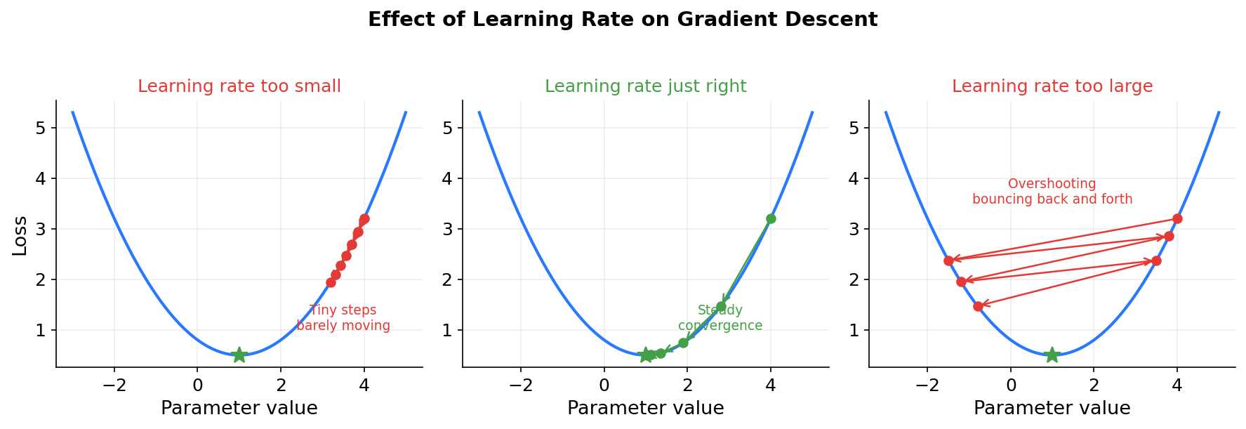
Applying this to the toy example from the previous section, with a learning rate of 0.1:

w1_new = 0.5   - 0.1 * 1.958    = 0.5   - 0.196  = 0.304
w2_new = -0.3  - 0.1 * (-3.264) = -0.3  + 0.326  = 0.026
w3_new = 1.2   - 0.1 * 0.816    = 1.2   - 0.082  = 1.118

Running the forward pass again with the new parameters to check whether the loss decreased:

h = 2.0 * 0.304 = 0.608
a = 0.608 * 0.026 = 0.0158
y = 0.0158 * 1.118 = 0.0177
L = (0.0177 - 1.0)^2 = (-0.9823)^2 = 0.9649

The loss dropped from 1.8496 to 0.9649 after a single gradient step. Over many such steps, the loss would keep decreasing.

In Part 1, I mentioned that the training data is split into batches of 1,024 sequences, each 4,096 tokens long, roughly 4 million tokens per batch. The reason for this is that the total training data for Llama 2 is 2 trillion tokens. Computing the loss on all 2 trillion tokens before taking a single update step would be impossibly slow and would require storing all the intermediate computations in memory.

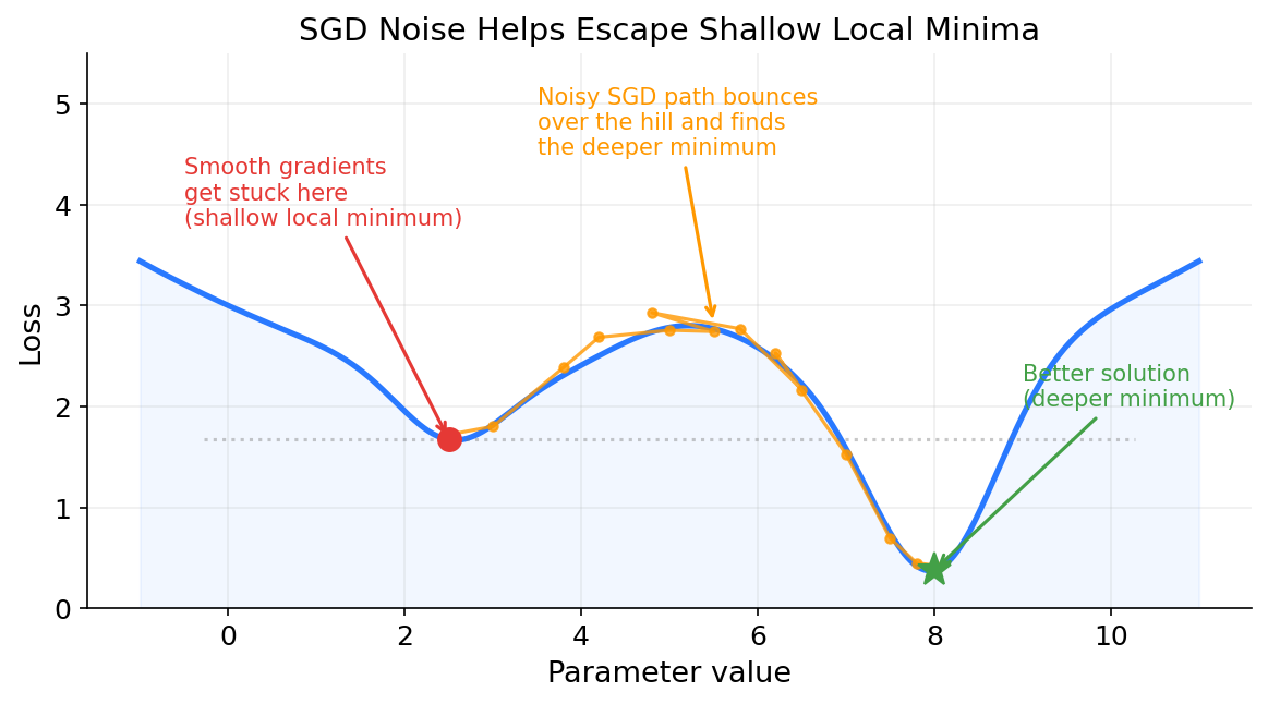
Instead, the model computes the loss and gradients on one batch at a time, updates the parameters, and moves to the next batch. This is called stochastic gradient descent (SGD). “Stochastic” just means random, because each batch is a random sample of the data. The update rule is exactly the same as above. The only difference is that the gradient comes from one batch instead of the full dataset.

The gradient from a single batch is noisy and might not point in the exact right direction. But on average, across many batches, it points the right way.

The noise actually helps. The loss landscape has many local minima, points where the loss is low relative to nearby parameter values but not the overall best. A perfectly smooth gradient computed from the entire dataset would follow a clean path downhill and settle into whatever local minimum it reaches first. At a local minimum the gradient is zero, so the optimizer has no signal to move and gets stuck. The noise from small batches adds randomness to each step, which can bounce the optimizer past shallow minima and toward deeper, better ones.

Going deeper: saddle points and sharp vs flat minima

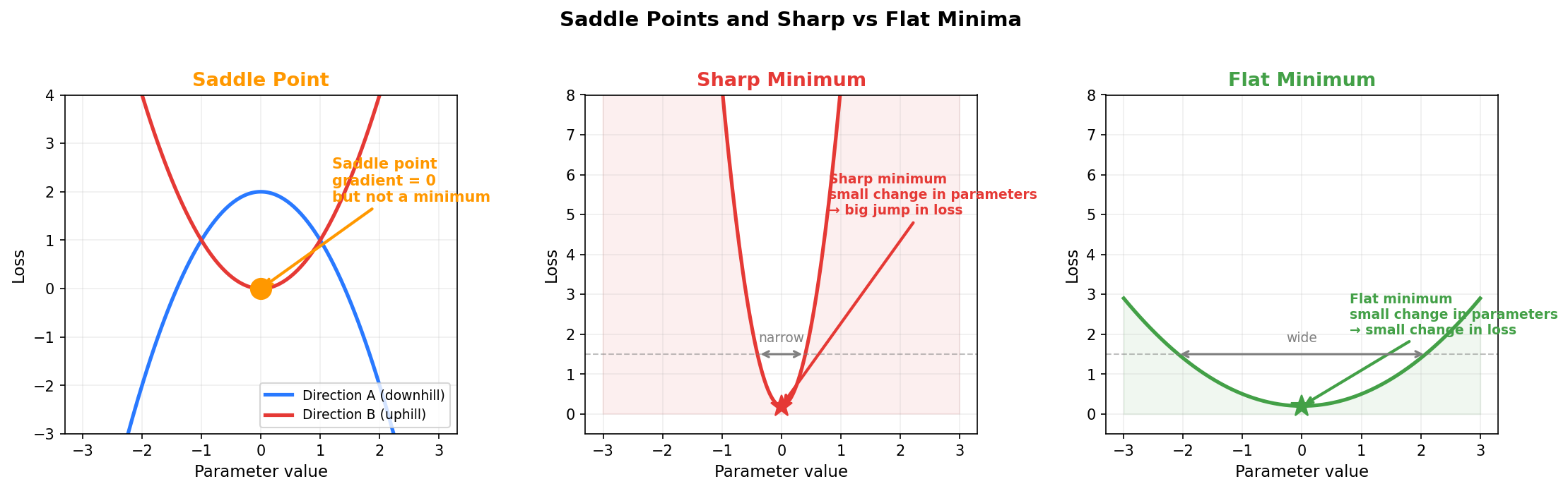
For deep networks with billions of parameters, the picture is more nuanced than just local minima. In a space with 8 billion dimensions, true local minima (where the loss is higher in every direction) are actually rare. Much more common are saddle points: points where the gradient is zero, but the loss curves downward in some dimensions and upward in others. Imagine sitting on a horse saddle. If you move forward or backward, you go downhill. If you move left or right, you go uphill. The gradient at the center of the saddle is zero in all directions, so a smooth optimizer would stop there thinking it found a minimum, even though there are directions it could move to get a lower loss. Noisy gradients from small batches naturally push the optimizer off saddle points because the random noise will eventually nudge it in one of the downhill directions.

There is another subtle benefit. Not all minima are equally good. Some minima are sharp: the loss is low at one specific set of parameter values but rises steeply if you change them even slightly. Others are flat: the loss stays low across a broad region of parameter values. Sharp minima tend to perform well on the training data but poorly on new data the model has never seen. Flat minima tend to perform well on both. This is the difference between memorization (learning the training data exactly) and generalization (learning patterns that transfer to new data). Noisy gradients tend to push the optimizer toward flatter minima because the noise makes it hard to settle precisely into a narrow, sharp valley. The optimizer keeps bouncing around until it finds a region broad enough to stay in despite the noise.

The Adam Optimizer

The gradient descent approach described above has a limitation: it uses the same learning rate for every parameter. Some parameters might need large updates and others might need tiny ones. A single learning rate cannot serve both well.

Adam (Adaptive Moment Estimation), introduced by Kingma and Ba, 2015, is the foundation of the optimizer used by most LLMs. In practice, many training runs use AdamW, a variant with decoupled weight decay, but the core mechanism is the same. Adam keeps track of two extra quantities for each parameter:

1. Momentum (first moment): a running average of the gradients over recent steps. If the gradient for a parameter has been consistently pointing in the same direction, momentum builds up and the parameter moves faster in that direction. Think of a ball rolling downhill. If the hill slopes consistently to the left, the ball accelerates. If the slope keeps changing direction, the ball slows down. Momentum smooths out noisy gradients and accelerates progress when the direction is consistent.

2. Adaptive learning rate (second moment): a running average of the squared gradients. Because the gradient is squared, the sign is removed: -0.5 and +0.5 both contribute 0.25. The second moment does not care about direction, only magnitude. It tracks how large the gradients have been recently. Parameters with consistently large gradients get a smaller effective learning rate (they are already changing a lot, so we slow them down). Parameters with small gradients get a larger effective learning rate (they need more help to make progress).

To see how the two moments work together, consider a parameter whose gradient oscillates between +5.0 and -5.0 every step. Momentum (first moment) averages to roughly zero because the positives and negatives cancel out, so the parameter barely moves. The second moment sees 25 every step (because 5^2 = 25), so it shrinks the learning rate. Both mechanisms are doing something useful: momentum says “the signal is contradictory, do not move,” and the adaptive rate says “and when you do move, take small steps, because this parameter is in a volatile region.”

Now consider a parameter with a consistent gradient of +5.0 every step. Momentum builds to 5.0, pushing hard in that direction. But the second moment also grows to 25 (since 5.0² = 25), and the update gets divided by sqrt(25) = 5.0. So the actual update is 5.0 / 5.0 = 1.0.

Compare this to a parameter with a consistent gradient of 0.01. Its momentum is 0.01, its second moment is 0.0001, and its update is 0.01 / sqrt(0.0001) = 0.01 / 0.01 = 1.0. Both parameters end up with updates of similar size, even though their raw gradients differ by 500x. The second moment acts as a built-in normalizer. Parameters with large gradients get their updates scaled down. Parameters with small gradients get their updates scaled up. Everyone moves at roughly the same pace.

Together, these two mechanisms let Adam tune each parameter independently. Parameters with steady, consistent gradients get larger updates. Parameters with volatile, noisy gradients get smaller ones.

Each of the model’s 8 billion parameters has its own m (momentum) and v (squared gradient average) values. That is 8 billion m values and 8 billion v values stored in memory. These are not part of the forward or backward pass. They are persistent state that sits alongside each parameter and only gets updated during the Adam step. After loss.backward() computes a gradient for every parameter across all 32 layers, Adam uses each parameter’s gradient to update that parameter’s m and v, and then updates the parameter itself. This happens for all 8 billion parameters at once.

This extra storage is why Adam uses more memory than plain gradient descent. SGD stores only the parameters themselves (8 billion numbers). Adam stores the parameters plus m plus v, so 3 values per parameter instead of one. For a model with 8 billion parameters at 4 bytes each, that is the difference between 32 GB (SGD) and 96 GB (Adam).

Now that we understand what Adam tracks and why, here is how the update rule works. It has four steps:

Step 1: Update the momentum. This blends the previous momentum with the current gradient. β1 controls how much history to keep. A higher value means more weight on past gradients:

m = β1 * m_prev + (1 - β1) * gradient

Step 2: Update the squared gradient average. This tracks how large gradients have been recently, which Adam uses to scale the learning rate per parameter. β2 controls how slowly this average changes:

v = β2 * v_prev + (1 - β2) * gradient^2

Step 3: Correct the bias. Since m and v are both initialized at zero before training starts, they are biased toward zero for the first several steps. The correction compensates for this by dividing by a term that depends on the step number t. At step 1: (1 - 0.9^1) = 0.1, so m_hat = m / 0.1, which multiplies m by 10x. At step 10: (1 - 0.9^10) = 0.65, so the correction is about 1.5x. At step 100: (1 - 0.9^100) = 0.99997, so m_hat ≈ m and the correction is effectively gone. The “hat” suffix is just mathematical convention for “corrected estimate”:

m_hat = m / (1 - β1^t)
v_hat = v / (1 - β2^t)

Step 4: Update the parameter. The momentum m_hat sets the direction and speed. Dividing by sqrt(v_hat) scales down parameters with large recent gradients and scales up parameters with small ones. ε is a tiny constant (typically 10^-8) added to prevent division by zero in the rare case where v_hat is exactly zero:

w_new = w_old - lr * m_hat / (sqrt(v_hat) + ε)

A Python pseudocode for Adam’s update:

# State: these persist across steps (initialized to 0 for each parameter)
m = 0  # momentum
v = 0  # squared gradient average

for t in range(1, num_steps + 1):
    gradient = compute_gradient(parameter)  # placeholder: in practice, loss.backward() computes all gradients at once

    m = beta1 * m + (1 - beta1) * gradient         # blend old momentum with new gradient
    v = beta2 * v + (1 - beta2) * gradient ** 2     # blend old average with new squared gradient

    m_hat = m / (1 - beta1 ** t)                    # bias correction
    v_hat = v / (1 - beta2 ** t)                    # bias correction

    parameter = parameter - lr * m_hat / (math.sqrt(v_hat) + epsilon)

Applying this to a single parameter across 4 training steps (each step uses a different batch of data), where the parameter’s gradient is 0.5, 0.3, 0.4, and -0.2 respectively. With β1 = 0.9, β2 = 0.999, lr = 0.01. The first three gradients are positive (all suggesting the parameter should decrease), and the fourth flips negative:

Step 1: gradient = 0.5
  m = 0.9 * 0 + 0.1 * 0.5       = 0.05
  v = 0.999 * 0 + 0.001 * 0.25  = 0.00025
  m_hat = 0.05 / (1 - 0.9^1)    = 0.05 / 0.1     = 0.500
  v_hat = 0.00025 / (1 - 0.999) = 0.00025 / 0.001 = 0.250
  update = 0.01 * 0.500 / (sqrt(0.250) + 1e-8) = 0.01 * 0.500 / 0.500 = 0.0100

Step 2: gradient = 0.3
  m = 0.9 * 0.05 + 0.1 * 0.3    = 0.075
  v = 0.999 * 0.00025 + 0.001 * 0.09 = 0.00034
  m_hat = 0.075 / (1 - 0.9^2)   = 0.075 / 0.19   = 0.395
  v_hat = 0.00034 / (1 - 0.999^2) = 0.00034 / 0.002 = 0.170
  update = 0.01 * 0.395 / (sqrt(0.170) + 1e-8) = 0.01 * 0.395 / 0.412 = 0.0096

Step 3: gradient = 0.4
  m = 0.9 * 0.075 + 0.1 * 0.4   = 0.1075
  v = 0.999 * 0.00034 + 0.001 * 0.16 = 0.00050
  m_hat = 0.1075 / (1 - 0.9^3)  = 0.1075 / 0.271 = 0.397
  v_hat = 0.00050 / (1 - 0.999^3) = 0.00050 / 0.003 = 0.167
  update = 0.01 * 0.397 / (sqrt(0.167) + 1e-8) = 0.01 * 0.397 / 0.409 = 0.0097

Step 4: gradient = -0.2  ← gradient flips direction
  m = 0.9 * 0.1075 + 0.1 * (-0.2) = 0.0768
  v = 0.999 * 0.00050 + 0.001 * 0.04 = 0.00054
  m_hat = 0.0768 / (1 - 0.9^4)  = 0.0768 / 0.344 = 0.223
  v_hat = 0.00054 / (1 - 0.999^4) = 0.00054 / 0.004 = 0.135
  update = 0.01 * 0.223 / (sqrt(0.135) + 1e-8) = 0.01 * 0.223 / 0.367 = 0.0061

A few observations from the walkthrough above:

• At step 1, raw momentum is 0.05 but the corrected value is 0.5. Without correction, the first update would be 10x too small and the model would barely learn anything during the first few hundred steps.
• At step 4, the gradient flips to -0.2, but momentum is still positive (0.223) because the previous three steps were positive. The update slows down instead of instantly reversing. Since each batch is a random sample, one batch might say “move this parameter left” while the overall trend is “move right.” Without momentum, the parameter would jitter back and forth every step. With momentum, it follows the trend and ignores the noise.
• Despite gradients ranging from -0.2 to 0.5, the updates are all around 0.006 to 0.01. In a real model, different parameters see very different gradient magnitudes. A parameter in the attention layer might consistently get gradients around 5.0, while one in the embedding layer might get 0.001. A single learning rate would be too large for the first (overshooting) and too small for the second (barely moving). Adam avoids this because each parameter’s update is scaled by its own gradient history. Large gradients get divided by a large number, small gradients by a small number, and the resulting updates end up at a similar scale.

The recommended defaults from the original paper are β1 = 0.9, β2 = 0.999, and ε = 10^-8. In PyTorch, using Adam is one line:

optimizer = torch.optim.Adam(model.parameters(), lr=1e-4)

Learning Rate Schedules

Adam adapts the effective learning rate per parameter, but there is still a base learning rate (lr in the formula above) that scales all updates. Using the same base learning rate from start to finish does not work well. Early in training the parameters are random, the loss is high, and the gradients are large and unstable. A high learning rate at this stage would cause the model to diverge. But later in training, once the model is close to a good solution, the same learning rate that worked in the middle of training is now too large and causes the model to overshoot and oscillate around the minimum instead of settling into it.

Most LLM training runs solve this with a learning rate schedule that changes the base learning rate over the course of training. The schedule typically has two phases. In the first phase, called warmup, training starts with a very small learning rate and gradually increases it over the first few thousand steps. This lets the model settle into a reasonable region of the loss landscape before taking bigger steps. In the second phase, the learning rate gradually decreases back down. The most common approach is cosine decay, where the learning rate follows a cosine curve from its peak down to near zero. The formula, from Loshchilov and Hutter, 2017, is:

lr(t) = lr_min + 0.5 * (lr_max - lr_min) * (1 + cos(π * t / T))

Here t is the current step (after warmup) and T is the total number of steps remaining after warmup. At t = 0, cos(0) = 1, so the learning rate is at its maximum. At t = T, cos(π) = -1, so it drops to lr_min. The idea is that early in training, when the model has only seen a few thousand batches, the parameters are still far from good values and larger steps help make fast progress. Later, after hundreds of thousands of batches, the model is getting close to a good solution and smaller steps let the parameters settle in without overshooting.

Llama 2 used 2,000 warmup steps followed by cosine decay down to 10% of the peak learning rate (Touvron et al. 2023).

Here is what the learning rate schedule looks like over the course of training:

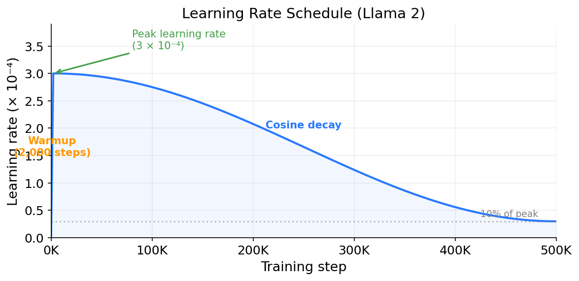
The steep ramp on the left is the warmup phase. Over the first 2,000 steps, the learning rate climbs from near zero to its peak value of 3×10⁻⁴. This is a tiny fraction of the full training run, less than half a percent of 500,000 total steps, but it is important. Without warmup, the model would start with a high learning rate while the gradients are still large and noisy from random initialization. That combination would push the parameters too far in unpredictable directions. Warmup avoids this by starting with a very small learning rate and gradually increasing it as the gradients stabilize. After warmup, the cosine decay takes over. The learning rate drops smoothly over the remaining 498,000 steps, reaching 10% of its peak value by the end. The curve is steeper in the middle and flattens out near the end, so the model takes progressively smaller steps as it approaches a good solution.

---

One Training Step, End to End

Putting it all together, here is the full cycle of a single training step:

1. Sample a batch of text from the training data.
2. Convert the text to token IDs using the tokenizer (the vocabulary was already built before training, as covered in Part 1).
3. Forward pass: feed the token IDs through the model (embedding lookup, 32 transformer layers, final linear layer, softmax). Get a probability distribution over the vocabulary for each position.
4. Compute cross-entropy loss: compare the predicted probabilities to the actual next tokens.
5. Backward pass: run backpropagation to compute the gradient for every parameter.
6. Optimizer step: use Adam to update all parameters.
7. Go back to step 1.

This loop repeats for the entire training run. Llama 2 trained on 2 trillion tokens with batches of about 4 million tokens, which works out to roughly 500,000 steps. Each step processes a batch of tokens, computes the loss, and updates the parameters. Step after step, the loss decreases and the model gets better at predicting the next token.

A Working Example

The code below trains a tiny transformer on a small piece of text. It is not a real LLM (that would need a GPU cluster), but the core training mechanics are the same as what we covered above. The architecture is simplified (it uses a basic TransformerEncoder instead of a full GPT-style decoder with RoPE, RMSNorm, and SwiGLU), but the training loop is the same. The forward pass, loss function, loss.backward(), and Adam optimizer all work the same way. The difference from real training would be scale, i.e. more parameters, more data, and more GPUs.

import torch
import torch.nn as nn

# --- Tiny dataset: a paragraph repeated ---
text = "the quick brown fox jumps over the lazy dog. the dog sleeps. the fox runs. "
text = text * 20  # repeat to have enough data. Real LLM training avoids repeating data
                   # because the model memorizes instead of learning general patterns.
                   # For our toy example, memorization is fine. If the loss goes down,
                   # the training loop is working correctly.

# --- Character-level tokenization (simple for demonstration) ---
vocab = sorted(set(text))                                      # all unique characters, sorted: [' ', '.', 'a', 'b', ...]
char_to_idx = {c: i for i, c in enumerate(vocab)}              # character → integer ID: {' ': 0, '.': 1, 'a': 2, ...}
idx_to_char = {i: c for i, c in enumerate(vocab)}              # integer ID → character (reverse lookup for decoding)
vocab_size = len(vocab)                                        # determines embedding table and output layer size
data = torch.tensor([char_to_idx[c] for c in text], dtype=torch.long)  # convert entire text to a tensor of token IDs
print(f"Vocab size: {vocab_size}, Dataset size: {len(data)} tokens")

# --- A tiny transformer model ---
torch.manual_seed(42)  # for reproducible output

# Uses TransformerEncoderLayer as a causal (decoder-only) stack
# by applying a triangular attention mask that prevents future token access.
class TinyTransformer(nn.Module):
    def __init__(self, vocab_size, embed_dim=64, num_layers=2, num_heads=2, max_seq_len=128):
        super().__init__()
        self.embedding = nn.Embedding(vocab_size, embed_dim)   # token → vector
        self.pos_embedding = nn.Embedding(max_seq_len, embed_dim)  # position → vector (learned, not RoPE)
        encoder_layer = nn.TransformerEncoderLayer(
            d_model=embed_dim, nhead=num_heads,
            dim_feedforward=128, dropout=0.0, batch_first=True # dropout=0 for memorization demo
        )
        self.transformer = nn.TransformerEncoder(encoder_layer, num_layers)
        self.fc = nn.Linear(embed_dim, vocab_size)             # project to vocabulary size

    def forward(self, x):
        seq_len = x.size(1)
        positions = torch.arange(seq_len, device=x.device)     # [0, 1, 2, ..., seq_len-1]
        x = self.embedding(x) + self.pos_embedding(positions)  # token vector + position vector, so "a" at position 0 differs from "a" at position 10

        # causal mask: each position can only attend to itself and earlier positions.
        # without this, position t could look at position t+1 which contains the answer.
        mask = nn.Transformer.generate_square_subsequent_mask(seq_len).to(x.device)
        x = self.transformer(x, mask=mask)
        return self.fc(x)                                      # output: logits for each position

model = TinyTransformer(vocab_size)
criterion = nn.CrossEntropyLoss()                             # takes raw logits, applies softmax internally
optimizer = torch.optim.Adam(model.parameters(), lr=1e-3)

# --- Training loop ---
seq_len, batch_size, num_steps = 32, 16, 500

for step in range(num_steps):
    # 1. Sample a random batch
    starts = torch.randint(0, len(data) - seq_len - 1, (batch_size,))
    inputs  = torch.stack([data[i : i + seq_len]     for i in starts])   # input tokens
    targets = torch.stack([data[i + 1 : i + seq_len + 1] for i in starts])  # shifted by 1: if input is positions 5-36, target is 6-37

    # 2. Forward pass
    logits = model(inputs)                                     # shape: [batch, seq_len, vocab_size]

    # 3. Compute loss. logits[:, t] is the prediction for targets[:, t],
    #    which is the next character after inputs[:, t].
    #    Reshape to [batch*seq_len, vocab_size] for cross-entropy.
    loss = criterion(logits.reshape(-1, vocab_size), targets.reshape(-1))

    # 4. Backward pass
    optimizer.zero_grad()                                      # clear gradients from previous step (without this, gradients accumulate)
    loss.backward()                                            # compute gradients for all parameters

    # 5. Optimizer step
    optimizer.step()                                           # update parameters using Adam

    if step % 100 == 0:
        print(f"Step {step:4d}  loss = {loss.item():.4f}")

# --- Generate text after training ---
model.eval()                                                   # switch to evaluation mode
with torch.no_grad():                                          # no need to track gradients
    prompt = torch.tensor([[char_to_idx['t']]])
    generated = prompt
    for _ in range(80):  # keep total length <= max_seq_len (128)
        logits = model(generated)
        next_token = torch.argmax(logits[0, -1, :]).unsqueeze(0).unsqueeze(0)  # greedy decoding
        generated = torch.cat([generated, next_token], dim=1)
    print("\nGenerated:", ''.join(idx_to_char[i.item()] for i in generated[0]))

Output (your exact numbers will vary due to random initialization):

Vocab size: 28, Dataset size: 1500 tokens
Step    0  loss = 3.3401
Step  100  loss = 1.4872
Step  200  loss = 0.7103
Step  300  loss = 0.3891
Step  400  loss = 0.2254

Generated: the quick brown fox jumps over the lazy dog. the dog sleeps. the fox runs. the qu

At step 0, the loss is about 3.34. That is close to log(28) = 3.33, which is the loss you would get from choosing uniformly at random between all 28 characters in the vocabulary. The model basically knows nothing yet.

By step 400, the loss has dropped to 0.23. That is a perplexity of e^0.23 = 1.26, meaning the model is almost never surprised by the next character. It has nearly memorized the training text and can reproduce it.

The generated text after training looks like the training data because we trained on a tiny repeated paragraph and the model memorized it. For a real LLM training on trillions of diverse tokens, the model cannot memorize everything and has to learn general patterns instead. But the training loop is the same: forward pass, loss, backprop, optimizer step. The difference is scale, which I will cover in Part 3.

---

Closing

In Part 3: From Toy Model to GPT, I will cover what happens when you scale this training loop to billions of parameters and trillions of tokens: parallelism across GPUs, what the model actually learns at each layer, and post-training alignment (fine-tuning, RLHF, DPO) that transforms a base model into the assistant you interact with.

---

Sources

Kingma and Ba, 2015. Adam: A Method for Stochastic Optimization

Loshchilov and Hutter, 2017. SGDR: Stochastic Gradient Descent with Warm Restarts

Touvron et al., 2023. Llama 2: Open Foundation and Fine-Tuned Chat Models

Meta, 2024. Llama 3 Model Card

Kaplan et al., 2020. Scaling Laws for Neural Language Models

---

<

Previous Post

How LLMs Work, Part 1: How LLMs Process Text

>

Blog Archive

Archive of all previous blog posts