How LLMs Work, Part 3: From Toy Model to GPT

In Part 1 I covered how text gets tokenized, embedded, and processed through the transformer architecture. In Part 2 I went through backpropagation, gradient descent, and the Adam optimizer. But there is a massive gap between a toy model that trains in seconds on a laptop and models like Llama 3 that train on thousands of GPUs for weeks. In this article I go through memory, parallelism, and training cost first, then what the model actually learns at different layers, and finally the post-training steps like fine-tuning and RLHF that turn a raw model into a usable assistant.

Scaling: What Changes When You Go from Toy to GPT

The Problem: One GPU Is Not Enough

The toy model from Part 2 fits in a few megabytes and trains in seconds. Real LLMs need significantly more.

Llama-3.1-8B has 8 billion parameters. As I discussed in the TurboQuant post, each parameter stored in FP16 (16-bit floating point) takes 2 bytes. So just storing the model parameters takes 8 billion x 2 bytes = 16 GB.

But during training, you need much more than just the parameters:

• Gradients: one gradient value for each parameter. Same size as the parameters: 16 GB.
• Optimizer states: Adam stores two extra values per parameter (the momentum and the squared gradient running averages). These are kept in FP32 (4 bytes each) for numerical precision. That is 8 billion x 4 bytes x 2 = 64 GB.
• Activations: the intermediate outputs of each layer. During the forward pass, every layer takes an input, transforms it, and produces an output. That output has to be stored in memory because backpropagation needs it later. In the toy example from Part 2, when we computed the gradient for w3, we needed the value of a = -0.3, which was computed during the forward pass. If we had not stored a, we would have had to recompute the entire forward pass up to that point just to get one gradient. Scaling that up to a real model with 32 layers, every layer produces intermediate outputs, and every one of those outputs needs to be kept in memory until backpropagation reaches that layer working backwards. The total memory depends on batch size and sequence length. For Llama-3.1-8B with a batch of 1,024 sequences of 4,096 tokens: each token at each layer is represented as a 4,096-dimensional vector (the embedding dimension), and all 32 layers’ outputs need to be stored. That is 1,024 sequences × 4,096 tokens × 4,096 numbers per token × 32 layers × 2 bytes (FP16) ≈ 1 TB. Activation checkpointing brings this down significantly by not storing every layer’s output. Instead, some outputs are recomputed during backpropagation, trading computation time for memory savings.

On top of this, training uses mixed precision. The forward and backward passes run in FP16 (16-bit floating point) because GPUs are much faster at FP16 math. But FP16 can only represent about 3-4 significant digits. When Adam computes a tiny update like 0.000003 and adds it to a parameter like 1.234, FP16 rounds the result back to 1.234. The update is lost completely because it is too small for FP16 to represent. To avoid this, training keeps a master copy of every parameter in FP32 (32-bit, about 7 significant digits), which adds another 32 GB. The training loop copies parameters from FP32 to FP16 for the fast forward and backward pass, computes gradients in FP16, and then applies the Adam update to the FP32 master copy where the precision is high enough to accumulate small changes. Without the FP32 master, small gradient updates would get rounded away and the model would eventually stop learning.

The forward pass does use slightly imprecise FP16 values, but a small rounding error in the forward pass barely affects the gradient. What matters is the accumulation of updates over thousands of steps. A single update of 0.000003 disappears in FP16, but 10,000 such updates add up to 0.03 in FP32, which is significant.

Add it all up and training an 8B parameter model requires roughly 130 to 160 GB of memory (the exact number depends on the training setup and precision choices). A single NVIDIA A100 GPU has 80 GB. It does not fit.

For Llama-3.1-70B with 70 billion parameters, these numbers are roughly 9x larger. Training it requires many GPUs working together.

Data Parallelism

The simplest way to use multiple GPUs is to put a copy of the entire model on every GPU and give each GPU a different batch of data.

Each GPU runs the forward pass on its own batch, computes the loss, runs backpropagation, and gets its own gradients. Then the GPUs communicate to average their gradients using an operation called all-reduce, where each GPU sends its gradients and receives the averaged result. After averaging, every GPU has the same gradient values and applies the same update, so all copies of the model stay in sync.

This is called data parallelism. It speeds up training because you process N batches in parallel (one per GPU) in the time it would take to process one. With 8 GPUs, you get roughly 8x the throughput.

The limitation is that every GPU needs to hold the full model. If the model does not fit on one GPU, data parallelism alone is not enough.

Model Parallelism

When the model itself is too large for a single GPU, you split it across multiple GPUs.

Tensor parallelism splits individual parameter matrices (also called weight matrices) inside each layer across GPUs. For example, a 4,096 × 4,096 matrix could be sliced into four pieces of 4,096 × 1,024, with each piece on a different GPU. Each GPU gets the same input, multiplies it by its slice, and produces a partial result (1,024 numbers instead of 4,096). The GPUs then share and combine their partial results to get the full output. This requires fast interconnects between GPUs because the communication happens within every layer.

To see how this works, here is a small example. A 3×4 matrix multiplied by a 4-dimensional input:

Full multiplication (one GPU):

                  [ 1 ]
[ 2  1  3  0 ]   [ 2 ]     Row 0: (2×1)+(1×2)+(3×3)+(0×4) = 13
[ 0  4  1  2 ] × [ 3 ]  =  Row 1: (0×1)+(4×2)+(1×3)+(2×4) = 19
[ 1  0  2  3 ]   [ 4 ]     Row 2: (1×1)+(0×2)+(2×3)+(3×4) = 19

With tensor parallelism across 2 GPUs, split the matrix by columns. GPU 0 takes columns 0-1, GPU 1 takes columns 2-3. Each GPU multiplies its columns with the corresponding input elements:

GPU 0 (columns 0-1, input[0] and input[1]):
  Row 0: (2×1)+(1×2) = 4
  Row 1: (0×1)+(4×2) = 8
  Row 2: (1×1)+(0×2) = 1

GPU 1 (columns 2-3, input[2] and input[3]):
  Row 0: (3×3)+(0×4) = 9
  Row 1: (1×3)+(2×4) = 11
  Row 2: (2×3)+(3×4) = 18

Combine (add partial results): [4+9, 8+11, 1+18] = [13, 19, 19]

We got the same answer and each GPU did half the work and stores only half the weight matrix in its memory. In practice, the split direction varies by layer and sometimes the input gets split too, but the idea is the same.

Pipeline parallelism assigns different layers to different GPUs. GPU 1 handles layers 1 through 8, GPU 2 handles layers 9 through 16, and so on. Data flows from GPU 1 to GPU 2 to GPU 3 like an assembly line. While GPU 2 is processing batch 1, GPU 1 can start on batch 2. The downside is that there are “bubbles” where some GPUs sit idle waiting for data, but clever scheduling (like interleaving micro-batches) can reduce this waste.

In practice, large training runs use all three: data parallelism across groups of GPUs, tensor parallelism within each group, and pipeline parallelism across stages. Meta trained Llama 3 on 16,384 H100 GPUs using a combination of all three strategies.

The Cost of Training

Training compute is measured in FLOPs (floating point operations). A single FLOP is one arithmetic operation like a multiplication or an addition. A useful approximation from Kaplan et al. 2020 estimates the total FLOPs for training a transformer with N parameters on D tokens as roughly 6 * N * D.

The 6 comes from counting operations at each parameter. In a matrix multiplication, each output number is a sum of products. For example, with a 3-element input: output = (input[0] × w[0]) + (input[1] × w[1]) + (input[2] × w[2]). Take a single parameter like w[0]. In the forward pass, it does one multiply (input[0] × w[0]) and one add (adding that product to the running sum). That is 2 operations per parameter in the forward pass.

In the backward pass (covered in Part 2), the model works backward from the loss to figure out how to adjust each parameter. At each layer, it needs to answer two questions.

The first question is: how much did each parameter contribute to the error? During the forward pass, w[0] was multiplied by input[0]. To figure out how much w[0] affected the final error, the model multiplies the error signal (how wrong the output was) by input[0] (the value that w[0] was applied to). This is one multiply and one add per parameter.

The second question is: how much did the input to this layer contribute to the error? This is needed because the input came from the previous layer, and that layer also needs to know how to adjust its own parameters. To compute this, the model multiplies the error signal by w[0] itself (the parameter value). Another multiply and add per parameter.

That gives 4 operations per parameter in the backward pass (2 for the parameter gradient, 2 for the input gradient).

Combined: 2 (forward) + 4 (backward) = 6 operations per parameter per token. Multiply by N parameters and D tokens and you get 6 * N * D.

For Llama 2 70B: 6 × 70 billion × 2 trillion = 8.4 × 10²³ FLOPs.

Meta reported that Llama 2 70B used 1,720,320 GPU-hours on A100 GPUs (Touvron et al. 2023). The A100 is NVIDIA’s data center GPU with 80 GB of memory and 312 TFLOPS of BF16 compute, designed specifically for large-scale machine learning workloads. Meta used 2,048 A100 GPUs for Llama 2 70B, which works out to roughly 35 days of continuous training. Translating GPU-hours to dollar costs depends on whether you own the hardware or rent it, and at what rate. Estimates for larger proprietary models are speculative since training costs are not typically disclosed.

Chinchilla Scaling Laws

So far I covered how much memory and compute training requires. But given a fixed compute budget, is it better to train a larger model on less data, or a smaller model on more data?

The Chinchilla paper (Hoffmann et al. 2022) from DeepMind showed that for a given compute budget, there is an optimal balance between model size and data size. They found that, for a fixed training compute budget, model size and training tokens should scale together. A common rule of thumb from Chinchilla is about 20 training tokens per model parameter. A 10 billion parameter model should therefore train on roughly 200 billion tokens.

Before Chinchilla, the trend was to train very large models on relatively little data. GPT-3 had 175 billion parameters but trained on about 300 billion tokens. By the 20x rule, a model that large would train on about 3.5 trillion tokens, over 10x more data.

After Chinchilla, the field shifted toward training models on far more data. Llama 2 70B trained on 2 trillion tokens, above the 1.4 trillion suggested by the 20x rule. Llama 3 pushed much further: its 70B model trained on over 15 trillion tokens.

The practical implication is that, for a fixed compute budget, you are often better off training a smaller model on more data than a larger model on too little data. A well-trained smaller model can outperform an undertrained larger model.

Data Quality and Preprocessing

The raw data that goes into training is not clean. Common Crawl alone contains billions of web pages, and a large portion of them are spam, duplicate content, boilerplate text, or low-quality machine-generated text. Training on this data directly would produce a model that generates the same kind of noise.

A significant part of the training pipeline is data cleaning and filtering. Typical steps include deduplication, language identification, quality filtering, boilerplate removal, PII mitigation, and sometimes filtering or measuring toxic and harmful content. The original LLaMA paper describes preprocessing Common Crawl with the CCNet pipeline: deduplicating text, using fastText for language identification, filtering low-quality pages with an n-gram language model, and training a classifier to prefer pages similar to Wikipedia references. Llama 2 continued this general approach with a new public-data mix, more robust cleaning, and efforts to remove sources likely to contain large amounts of personal information.

The mix of data sources also matters. Training exclusively on web text produces a model that sounds like the internet. Mixing in books, scientific papers, code, and curated datasets like Wikipedia produces a more well-rounded model. The Pile dataset was specifically designed for this: it combines 22 different sources in carefully chosen proportions. Getting the data mix right is increasingly recognized as a first-order decision in LLM training, often as important as architecture or optimizer choices.

What the Model Actually Learns

After training on trillions of tokens, the model’s 8 billion parameters are no longer random. They encode patterns learned from the data. Researchers have been studying what exactly those patterns look like at each layer.

Layers Learn Different Things

Researchers have studied what different transformer layers learn using probing experiments. The idea is to freeze the model, take the internal vectors from each layer, and train a small classifier to see what information can be decoded from those vectors.

Tenney et al. 2019 did this with BERT (a transformer model from Google) and found that its layers roughly follow the classical NLP pipeline. Lower layers capture surface and local syntactic information, such as part-of-speech patterns (figuring out that “cat” is a noun and “sat” is a verb). Middle layers capture richer syntactic and semantic relationships, such as dependencies, entity information, and semantic roles (figuring out that “cat” is an animal and “mat” is a surface). Later layers capture more global information, including coreference and discourse-level context.

This does not mean each layer has a clean job description. The boundaries are fuzzy, and information is distributed across many layers. A probe also shows only that information is present in a layer’s vectors, not necessarily that the model uses it directly. But the broad trend is consistent: as representations move upward through the network, they tend to become more abstract and more shaped by the model’s final prediction task.

Emergent Abilities

Some benchmark capabilities appear only after models reach a certain scale. Below that scale, measured performance can look close to random. Above it, performance may rise sharply.

Wei et al. 2022 collected several examples of this pattern and called them emergent abilities.

One example is few-shot arithmetic. In the GPT-3 paper, the 175B-parameter model reached about 80% accuracy on 3-digit addition when shown examples in the prompt. Much smaller GPT-3 variants performed far worse; the 13B model was around single-digit accuracy on the same task. Since GPT-3 did not test many model sizes between 13B and 175B, we know the jump happened somewhere in that range, but not exactly how sharp the transition really was.

Another example is chain-of-thought prompting. Wei et al. showed that giving large models examples with intermediate reasoning steps improves performance on multi-step reasoning tasks such as math word problems. Smaller models often do not benefit much from this prompting style. A related technique, zero-shot chain-of-thought (Kojima et al. 2022), uses prompts like “Let’s think step by step” to elicit similar reasoning behavior without examples.

There is active debate about whether these are true emergent properties or artifacts of measurement. Schaeffer et al. 2023 argued that sudden emergence often depends on the metric used. With exact-match accuracy, partial progress is invisible until the model starts getting the full answer right, making improvement look sudden. With smoother metrics, the same improvement can look more gradual.

Either way, scale matters. Larger models trained with more compute and data tend to perform better across a wider range of tasks. The debate is mostly about whether the improvement is truly sudden or whether our benchmarks make gradual progress look sudden.

Memorization vs. Generalization

A common question is whether the model just memorizes its training data.

The answer is both yes and no.

Models do memorize some training data verbatim, especially sequences that are repeated many times or have unusual structure, such as famous quotes, code, license text, logs, IDs, or contact information. Carlini et al. 2021 showed that GPT-2 could be prompted to emit hundreds of verbatim sequences from its training data, including public personally identifiable information, IRC conversations, code, and UUIDs. Later work found that memorization increases with model size, duplicated data, and the amount of prompt context provided.

But models also generalize. They can produce coherent continuations for prompts that never appeared exactly in training, combine ideas from different contexts, and apply learned patterns to new examples. If all they did was memorize, they would only reproduce stored passages, not adapt flexibly to new wording and new combinations of ideas.

The balance between memorization and generalization depends on model size, data quality, duplication, and training duration. Larger models can memorize more individual sequences, but they also tend to generalize better. The two are not opposites. The same learned representations that let a model reproduce familiar text can also help it produce novel text that follows the patterns of language.

After Pre-training: Fine-tuning and RLHF

Everything described so far, forward pass, loss function, backpropagation, gradient descent, and scaling, produces what is called a base model (also called a pre-trained model).

The Base Model Problem

A base model is very good at predicting the next token. If you give it “The capital of France is,” it will likely output “Paris.” It has absorbed enormous amounts of knowledge from its training data.

But a base model is not an assistant. It does not follow instructions. If you type “Write me a poem about cats,” a base model might continue with “and dogs. The poem should be at least 10 lines long and include the words…” because it is just predicting what text would come next on the internet. And on the internet, text that starts with “Write me a poem about cats” is often followed by more instructions (from a homework assignment or a forum post), not the poem itself.

To turn a base model into an assistant that can follow instructions and hold conversations, the most common approach involves two additional training stages (though the exact pipeline varies, some teams use only SFT, others use DPO, rejection sampling, or other variants).

Supervised Fine-Tuning (SFT)

The first step is supervised fine-tuning (SFT). You take the base model and continue training it, but now on a curated dataset of (instruction, response) pairs.

For example:

Instruction: Write a haiku about the ocean.
Response:    Waves crash on the shore
             Salt and foam in morning light
             The tide pulls away

The training process is the same as pre-training, forward pass, loss, backward pass, AdamW update. The difference is the data. Instead of random internet text, the model trains on thousands of curated examples where each example is an instruction paired with a good response. This data comes from a very different source than pre-training data. Instead of scraping the web, companies hire human annotators to write instruction-response pairs following specific quality guidelines. Some teams also convert existing NLP datasets (like question answering or summarization tasks) into instruction-response format, or use a stronger model like GPT-4 to generate responses that are then used to train a smaller model. The scale is much smaller than pre-training, typically tens of thousands to hundreds of thousands of examples rather than trillions of tokens. Quality matters far more than quantity at this stage.

One difference from pre-training is that the loss is computed only on the response tokens, not the instruction tokens. During pre-training, the model learns to predict every token in the text. But during SFT, we do not want the model to learn to predict the instruction itself. We want it to take the instruction as given and learn to produce a good response. If the loss included the instruction tokens, the model would spend training capacity learning to predict things like “Write a haiku about the ocean,” which is not useful. By masking out the instruction tokens, all of the learning signal goes toward improving the quality of the response.

The forward pass is the same as pre-training. The model processes the full sequence, instruction and response together, because it needs the instruction as context. It produces predictions at every position, but the loss only counts the response positions.

Position:   0     1    2     3     4    5      6    7     8    9    10   11
Token:     Write  a  haiku about  the ocean   |  Waves crash  on  the shore
Loss:        ✗    ✗    ✗     ✗     ✗    ✗     ✗    ✓     ✓    ✓    ✓    ✓

Cross-entropy loss is computed at the ✓ positions. The ✗ positions are skipped, and gradients flow only from the response tokens.

The model after SFT can follow instructions, but it does not have a good sense of what makes one response better than another. SFT teaches format (respond to questions, follow instructions), but not judgment. If you ask “How do I pick a lock?”, an SFT model might answer helpfully because it learned to follow instructions. It does not know that some instructions should not be followed. If you ask “Explain quantum computing,” it might produce a technically accurate but 2,000-word answer when a concise 200-word answer would be more useful. The model has no signal for which style of response a human would actually prefer. That is what the next step addresses.

Reinforcement Learning from Human Feedback (RLHF)

The second step is RLHF (Reinforcement Learning from Human Feedback). The approach builds on Christiano et al. 2017, which introduced deep reinforcement learning from human preferences. It was later applied to language models in work such as Ziegler et al. 2019 and Stiennon et al. 2020, and then popularized for broad instruction following by InstructGPT (Ouyang et al. 2022). Instead of just showing the model what a good response looks like, RLHF teaches it what humans prefer. It works in three phases.

In the first phase, the team collects comparison data. The SFT model is given a prompt and generates several different responses. Human evaluators see these responses and rank them from best to worst. For example, given the prompt “Explain gravity to a 5-year-old,” the model might generate four responses. A human ranks them and says response 3 is best, then response 1, then response 4, then response 2.

In the second phase, a reward model is trained. This is a separate neural network that takes a prompt and a response and outputs a single number representing how good the response is. It is trained on the human ranking data from the first phase, learning to assign higher scores to responses that humans preferred and lower scores to responses they did not.

In the third phase, the language model is optimized using PPO (Proximal Policy Optimization), a reinforcement learning algorithm. The language model is given a prompt and generates a response. The reward model scores the response. PPO updates the language model to increase the expected reward, while also adding a penalty if the model drifts too far from the SFT model. This constraint is important. Without it, the model can exploit flaws in the reward model and produce degenerate outputs that receive high reward but are not actually useful to humans. This loop repeats over many prompts.

The reward model itself is usually another transformer, often initialized from the base model or SFT model. It takes the prompt and response as input, runs a normal forward pass through its own layers, and uses a final reward head to output a single scalar score instead of a probability distribution over the vocabulary. During the second phase, this reward model is trained on human preference data so that preferred responses receive higher scores than rejected responses. During the third phase, the reward model is frozen and used only as a scoring function while PPO updates the language model.

The key difference from pre-training is where the training signal comes from. In pre-training and SFT, the signal is per-token: “you predicted token X, the correct token was Y.” In RLHF, the signal is per-response: “you generated this entire response, the reward model scored it 0.8, adjust yourself to score higher next time.” The gradients still flow through the same layers, same attention, same feedforward, same Adam update. Only the source of the training signal changes.

Direct Preference Optimization (DPO)

RLHF works, but it has a lot of moving parts. You need to train a separate reward model, PPO is finicky to tune, and the whole pipeline is complex to maintain.

Rafailov et al. 2023 introduced DPO (Direct Preference Optimization) as a simpler alternative. The idea is to skip the explicit reward model and train the language model directly on preference data.

The training data for DPO looks like this: for a given prompt, you have two responses, one that a human preferred and one that was rejected. For example, given the prompt “Explain gravity to a 5-year-old,” response A might say “Gravity is what makes things fall down when you drop them,” while response B might say “Gravity is the curvature of spacetime caused by mass-energy density.” A human annotator prefers response A for this audience.

DPO’s loss function uses this pair to push the model toward the preferred response and away from the rejected one. In language-model terms, it makes the model assign higher probability to the sequence of tokens in response A than to the sequence of tokens in response B, given the same prompt.

But it does this relative to a frozen reference model, usually the SFT model. The reference model acts as an anchor. DPO is not saying, “Change the model as much as possible until it always chooses A-style answers.” It is saying, “Prefer A over B more than the reference model does, but do not drift too far from the reference model’s behavior.” This plays a similar role to PPO’s drift constraint, but DPO achieves it with a single loss function instead of a separate reward model and reinforcement-learning loop.

No separate reward model, no PPO loop, just a modified loss function on the same kind of preference data.

DPO is simpler to implement and often competitive with PPO-based RLHF on standard preference-tuning benchmarks. Zephyr uses SFT followed by DPO, avoiding PPO entirely. Llama 3 uses DPO alongside supervised fine-tuning and rejection sampling as part of its post-training pipeline.

The Full Pipeline

The diagram below shows how all the stages fit together. Pre-training produces a base model that can predict the next token but cannot follow instructions. SFT teaches it to respond to instructions. Then either RLHF (with a reward model and PPO) or DPO aligns the model’s responses with human preferences. The result is the chat model you interact with.

Next Up

This article covered the training side of large language models. How much memory they need, how training is split across GPUs, why training is so expensive, how scaling laws shape model and data choices, why data quality matters, what different layers learn, and how post-training alignment turns a base model into an assistant.

The next step is inference, running the trained model to generate text. In Part 4, I will cover how generation works one token at a time, why the KV cache matters, and how decoding strategies like temperature, top-k, and top-p control the style and diversity of the output.

How LLMs Work, Part 2: How LLMs Learn

In Part 1, I covered tokenization and the forward pass: how text becomes numbers, and how those numbers flow through a transformer to produce predictions. But a model with random parameters makes random predictions. It needs to learn.

In this article, we will explore the loss function that measures how wrong the model is, backpropagation that computes gradients, and the optimizers (SGD, Adam) that adjust billions of parameters. I go through gradient descent and learning rate schedules with worked examples, and finish with a complete training loop you can run yourself.

The Loss Function: Measuring How Wrong the Model Is

Let’s go back to the training sentence from earlier: “The cat sat on the mat.” The model just predicted probabilities for each possible next token after “The cat sat on the.” The actual next word in the training data is “mat,” but the model assigned “mat” a probability of only 0.233 (23.3%) and gave “rug” 63.4%. The model got it wrong. We need a way to measure how wrong it was. That measurement is called the loss.

The loss function used by virtually all language models is cross-entropy loss. The formula is as follows:

loss = -log(probability of the correct token)

Here log is the natural logarithm (base e). Computing the loss for our example: The correct token is “mat”, and the model gave it probability 0.233.

loss = -log(0.233) = -(-1.457) = 1.457

What if the model had been more confident and correct? If it gave “mat” probability 0.95:

loss = -log(0.95) = 0.051

That gives a loss of 0.051, compared to 1.457 when the model assigned only 23.3% to “mat.” The model is being rewarded for being confident in the right answer.

What if the model had been very wrong? If it gave “mat” probability 0.01:

loss = -log(0.01) = 4.605

Very high. The loss function heavily penalizes confident wrong predictions.

Here is a table showing how loss changes with the model’s confidence in the correct answer:

As the pattern shows, loss is 0 when the model assigns probability 1.0 to the correct token. As the probability of the correct token drops toward 0, the loss climbs toward infinity. The loss function is small when the model gives the correct token a high probability, but if the model gives the correct token a very low probability (meaning it was very wrong), the loss is very large.

The goal of training is to minimize the average loss across all tokens in the training data. If we have a dataset with one million tokens, we compute the loss for each token’s prediction, add them all up, and divide by one million. We want that average number to be as small as possible.

There is one more metric you will see in LLM papers: perplexity. It is defined as:

perplexity = e^(average loss)

If the average cross-entropy loss across all tokens in a dataset is 2.5, then perplexity = e^2.5 = 12.18. Intuitively, perplexity measures how many tokens the model is “confused between” on average. A perplexity of 12 means the model is, on average, as uncertain as if it were choosing randomly between 12 equally likely tokens. Lower perplexity means a better model. Researchers report both because they are two ways of looking at the same thing: loss is what the optimizer actually minimizes (it is the raw number the math works with), and perplexity gives a more human-interpretable scale. “The model is confused between 12 tokens on average” is easier to reason about than “the loss is 2.5.”

Backpropagation: How the Model Learns from Mistakes

We now have a number (the loss) that tells us how wrong the model is. The question is: how do we adjust the model’s parameters to make the loss smaller?

There are billions of parameters. We cannot just try random changes and hope for the best. We need a systematic way to figure out which direction to adjust each parameter.

Gradients: Which Way Is Downhill?

Imagine you are standing on a hilly landscape and you want to get to the lowest point. You are blindfolded, so you cannot see the whole landscape. But you can feel the slope of the ground under your feet. If the ground slopes downward to your left, you step left. If it slopes downward in front of you, you step forward. Each step takes you a little lower.

A gradient is the mathematical version of “the slope under your feet.” For each parameter in the model, the gradient tells you: if I increase this parameter by a tiny amount, does the loss go up or down, and by how much?

Concretely: suppose one of the 8 billion parameters in the model is a number w = 0.5. The loss right now is 1.457 (from our “mat” example). We want to know: if we change w by a tiny amount, does the loss go up or down? We cannot just try every possible change because there are 8 billion parameters. Instead, we compute the gradient using calculus (the chain rule, covered in the next section). The gradient is a single number that tells us the answer. Suppose the gradient of the loss with respect to w comes out to +0.3. The sign tells us the direction: positive means increasing w makes the loss worse, negative means increasing w makes the loss better. The magnitude tells us how sensitive the loss is to this parameter. To see what +0.3 means concretely, imagine nudging w upward by a tiny amount, say 0.001. The gradient says the loss would change by approximately gradient × nudge = 0.3 × 0.001 = 0.0003. Since the gradient is positive, the loss goes up by 0.0003. That is bad, because we want the loss to go down. So we should nudge w in the other direction, downward.

That is the entire idea:

• Positive gradient means increasing this parameter makes the loss worse. Decrease it.
• Negative gradient means increasing this parameter makes the loss better. Increase it.
• Large gradient means this parameter has a big effect on the loss right now.
• Gradient near zero means this parameter barely matters for this particular prediction.

To visualize how gradients work, imagine a model with just one parameter w. In reality there are 8 billion parameters, but we can only draw a 2D chart, so we simplify down to one. The x-axis is the value of that parameter. The y-axis is the loss the model would produce if the parameter had that value (with all other parameters held fixed). The result is a curve, and somewhere on that curve is a low point where the loss is smallest. That is where we want the parameter to end up.

The gradient is the slope of this curve at the current parameter value. If the slope tilts upward to the right (positive gradient), it means increasing the parameter would increase the loss, so we should decrease it. If the slope tilts downward to the right (negative gradient), increasing the parameter would decrease the loss, so we should increase it. The steeper the slope, the larger the gradient, and the bigger the step we take.

Real models have billions of parameters, and computing the gradient for a parameter buried 20 layers deep in the model, with millions of operations between it and the loss, is not straightforward. That is where the chain rule comes in.

The Chain Rule

The model is a chain of operations: embedding lookup, then layer 1, then layer 2, all the way through layer 32, then the final linear layer (the matrix multiplication that converts the 4,096-number vector into 128,256 logits, as described in the “Predicting the Next Token” section), then softmax, then the loss computation. Each operation takes the output of the previous one as input.

The chain rule from calculus says: if you have a composition of functions, the derivative (gradient) of the whole chain is the product of the derivatives of each step. Written as a formula:

dL/dw1 = (dL/dy) * (dy/da) * (da/dh) * (dh/dw1)

Reading right to left: dh/dw1 is “how much does changing w1 affect h?” Then da/dh is “how much does changing h affect a?” And so on, all the way to dL/dy, “how much does changing y affect the loss?” Multiply them all together and you get the total effect of w1 on the loss, even though w1 and the loss are many steps apart.

In the forward pass, data flows forward: input → layers → prediction → loss. Backpropagation goes the other way. It applies this chain rule backwards through the model, from the loss all the way back to the first layer, computing the gradient for every single parameter. The “back” in backpropagation refers to this direction: you start at the loss and work backwards toward the input, computing one derivative at each step.

One challenge with deep networks is that this chain of multiplied derivatives can shrink as it passes through many layers. To understand why, consider how the chain rule works across layers. To compute the gradient for a parameter in layer 1, the chain rule must multiply derivatives through every layer between layer 1 and the loss: dL/dw = (dL/d_layer32) × (d_layer32/d_layer31) × ... × (d_layer2/d_layer1) × (d_layer1/dw). If each layer’s derivative is 0.8, then 0.8^32 = 0.001, and the gradient reaching layer 1 is a thousand times smaller than the gradient at layer 32. As a result, the early layers barely learn. This is called the vanishing gradient problem.

Transformers address this with residual connections (also called skip connections). Each of the 32 transformer layers from Part 1 (attention followed by feedforward) takes a vector as input and produces a modified vector as output. For the token “the” in “The cat sat on the,” layer 1 receives the raw embedding vector, runs attention to blend in context from “cat,” “sat,” and “on,” then runs the feedforward network to create new features. The result is a modified vector that becomes layer 2’s input. Layer 2 does the same thing, refining the vector further, and passes its output to layer 3, and so on through all 32 layers. The residual connection is about how each layer combines its own computation with what it received.

Instead of each layer computing output = f(input), where f is that layer’s attention and feedforward processing, it computes output = input + f(input). The layer adds its transformation to the original input rather than replacing it. This works because the layer does not need to learn the entire output from scratch. It only needs to learn what to change. If a layer has nothing useful to add, f(input) can learn to output values close to zero, and the input passes through mostly unchanged. This makes training easier because the layer starts from a useful default (pass the input through) rather than having to learn everything from scratch. If it does learn something useful, it adds that on top. Mathematically, the derivative of input + f(input) with respect to input is 1 + f'(input). That 1 gives the gradient a direct path to flow backward without being multiplied down by the layer’s internal operations.

For example, suppose a layer receives an input vector where one value is 5.0, and the layer’s transformation f produces 0.3 for that position. Without a residual connection, the output is just 0.3, and the derivative through this layer is f'(input), which might be something small like 0.1. With a residual connection, the output is 5.0 + 0.3 = 5.3, and the derivative is 1 + 0.1 = 1.1. The gradient flowing backward through this layer barely shrinks. Without residual connections and a derivative of 0.1 per layer, 32 layers gives 0.1^32, which is effectively zero. With residual connections, the derivative per layer is closer to 1 (for example 0.95 or 1.05), so the gradient passes through all 32 layers without vanishing.

A Toy Example

Let us walk through backpropagation on a tiny “network” with just 3 parameters to see how the math works in practice.

Setup:

• Input: x = 2.0
• Three parameters: w1 = 0.5, w2 = -0.3, w3 = 1.2
• The forward pass computes: h = x * w1, then a = h * w2, then y = a * w3
• The target output is 1.0
• Loss function: squared error, L = (y - target)^2

Forward pass:

h = x * w1 = 2.0 * 0.5 = 1.0
a = h * w2 = 1.0 * (-0.3) = -0.3
y = a * w3 = (-0.3) * 1.2 = -0.36
L = (y - target)^2 = (-0.36 - 1.0)^2 = (-1.36)^2 = 1.8496

The loss is 1.8496. Now let us work backwards to compute the gradient for each parameter.

Backward pass:

Start at the loss. The derivative of L = (y - target)^2 with respect to y is:

dL/dy = 2 * (y - target) = 2 * (-1.36) = -2.72

Now go back one step. y = a * w3, so:

dy/dw3 = a = -0.3
dL/dw3 = dL/dy * dy/dw3 = (-2.72) * (-0.3) = 0.816

dy/da = w3 = 1.2
dL/da = dL/dy * dy/da = (-2.72) * 1.2 = -3.264

Go back one more step. a = h * w2, so:

da/dw2 = h = 1.0
dL/dw2 = dL/da * da/dw2 = (-3.264) * 1.0 = -3.264

da/dh = w2 = -0.3
dL/dh = dL/da * da/dh = (-3.264) * (-0.3) = 0.979

One more step back. h = x * w1, so:

dh/dw1 = x = 2.0
dL/dw1 = dL/dh * dh/dw1 = 0.979 * 2.0 = 1.958

The gradients are:

That is backpropagation. We started at the loss and worked backwards through each operation, multiplying derivatives along the way, until we had the gradient for every parameter.

Computing Gradients at Scale

For a model with 8 billion parameters and dozens of different operations (matrix multiplications, attention, layer normalization, nonlinear activations), manual gradient computation is impossible.

Frameworks like PyTorch and JAX use a system called autograd (automatic differentiation). As the forward pass runs, the framework records every operation in a computational graph. It tracks which inputs produced which outputs, and what operation was applied. When the forward pass is complete and the loss is computed, you call one function, loss.backward() in PyTorch, and it walks the computational graph in reverse, applying the chain rule automatically to compute the gradient for every parameter.

Calling loss.backward() produces gradients for all 8 billion parameters, by doing the same chain-rule walk we saw in the example above, applied across every operation in the graph.

Gradient Descent and Optimizers

At this point we have the gradients for every parameter. Each gradient tells us which direction to adjust that parameter to reduce the loss. The next step is to actually update them.

Gradient Descent

The simplest update rule is called gradient descent. For each parameter, subtract the gradient multiplied by a small number called the learning rate:

w_new = w_old - learning_rate * gradient

The minus sign is because the gradient points in the direction of increasing loss, and we want to decrease it.

The learning rate controls how big each step is. It is a small number, typically between 0.0001 and 0.001 for LLM training. If the learning rate is too large, the model overshoots: it makes such big changes that the loss actually goes up instead of down, and training becomes unstable or diverges. If the learning rate is too small, training works but takes an impractical amount of time because each step barely moves the parameters.

Applying this to the toy example from the previous section, with a learning rate of 0.1:

w1_new = 0.5   - 0.1 * 1.958    = 0.5   - 0.196  = 0.304
w2_new = -0.3  - 0.1 * (-3.264) = -0.3  + 0.326  = 0.026
w3_new = 1.2   - 0.1 * 0.816    = 1.2   - 0.082  = 1.118

Running the forward pass again with the new parameters to check whether the loss decreased:

h = 2.0 * 0.304 = 0.608
a = 0.608 * 0.026 = 0.0158
y = 0.0158 * 1.118 = 0.0177
L = (0.0177 - 1.0)^2 = (-0.9823)^2 = 0.9649

The loss dropped from 1.8496 to 0.9649 after a single gradient step. Over many such steps, the loss would keep decreasing.

In Part 1, I mentioned that the training data is split into batches of 1,024 sequences, each 4,096 tokens long, roughly 4 million tokens per batch. The reason for this is that the total training data for Llama 2 is 2 trillion tokens. Computing the loss on all 2 trillion tokens before taking a single update step would be impossibly slow and would require storing all the intermediate computations in memory.

Instead, the model computes the loss and gradients on one batch at a time, updates the parameters, and moves to the next batch. This is called stochastic gradient descent (SGD). “Stochastic” just means random, because each batch is a random sample of the data. The update rule is exactly the same as above. The only difference is that the gradient comes from one batch instead of the full dataset.

The gradient from a single batch is noisy and might not point in the exact right direction. But on average, across many batches, it points the right way.

The noise actually helps. The loss landscape has many local minima, points where the loss is low relative to nearby parameter values but not the overall best. A perfectly smooth gradient computed from the entire dataset would follow a clean path downhill and settle into whatever local minimum it reaches first. At a local minimum the gradient is zero, so the optimizer has no signal to move and gets stuck. The noise from small batches adds randomness to each step, which can bounce the optimizer past shallow minima and toward deeper, better ones.

Going deeper: saddle points and sharp vs flat minima

For deep networks with billions of parameters, the picture is more nuanced than just local minima. In a space with 8 billion dimensions, true local minima (where the loss is higher in every direction) are actually rare. Much more common are saddle points: points where the gradient is zero, but the loss curves downward in some dimensions and upward in others. Imagine sitting on a horse saddle. If you move forward or backward, you go downhill. If you move left or right, you go uphill. The gradient at the center of the saddle is zero in all directions, so a smooth optimizer would stop there thinking it found a minimum, even though there are directions it could move to get a lower loss. Noisy gradients from small batches naturally push the optimizer off saddle points because the random noise will eventually nudge it in one of the downhill directions.

There is another subtle benefit. Not all minima are equally good. Some minima are sharp: the loss is low at one specific set of parameter values but rises steeply if you change them even slightly. Others are flat: the loss stays low across a broad region of parameter values. Sharp minima tend to perform well on the training data but poorly on new data the model has never seen. Flat minima tend to perform well on both. This is the difference between memorization (learning the training data exactly) and generalization (learning patterns that transfer to new data). Noisy gradients tend to push the optimizer toward flatter minima because the noise makes it hard to settle precisely into a narrow, sharp valley. The optimizer keeps bouncing around until it finds a region broad enough to stay in despite the noise.

The Adam Optimizer

The gradient descent approach described above has a limitation: it uses the same learning rate for every parameter. Some parameters might need large updates and others might need tiny ones. A single learning rate cannot serve both well.

Adam (Adaptive Moment Estimation), introduced by Kingma and Ba, 2015, is the foundation of the optimizer used by most LLMs. In practice, many training runs use AdamW, a variant with decoupled weight decay, but the core mechanism is the same. Adam keeps track of two extra quantities for each parameter:

1. Momentum (first moment): a running average of the gradients over recent steps. If the gradient for a parameter has been consistently pointing in the same direction, momentum builds up and the parameter moves faster in that direction. Think of a ball rolling downhill. If the hill slopes consistently to the left, the ball accelerates. If the slope keeps changing direction, the ball slows down. Momentum smooths out noisy gradients and accelerates progress when the direction is consistent.

2. Adaptive learning rate (second moment): a running average of the squared gradients. Because the gradient is squared, the sign is removed: -0.5 and +0.5 both contribute 0.25. The second moment does not care about direction, only magnitude. It tracks how large the gradients have been recently. Parameters with consistently large gradients get a smaller effective learning rate (they are already changing a lot, so we slow them down). Parameters with small gradients get a larger effective learning rate (they need more help to make progress).

To see how the two moments work together, consider a parameter whose gradient oscillates between +5.0 and -5.0 every step. Momentum (first moment) averages to roughly zero because the positives and negatives cancel out, so the parameter barely moves. The second moment sees 25 every step (because 5^2 = 25), so it shrinks the learning rate. Both mechanisms are doing something useful: momentum says “the signal is contradictory, do not move,” and the adaptive rate says “and when you do move, take small steps, because this parameter is in a volatile region.”

Now consider a parameter with a consistent gradient of +5.0 every step. Momentum builds to 5.0, pushing hard in that direction. But the second moment also grows to 25 (since 5.0² = 25), and the update gets divided by sqrt(25) = 5.0. So the actual update is 5.0 / 5.0 = 1.0.

Compare this to a parameter with a consistent gradient of 0.01. Its momentum is 0.01, its second moment is 0.0001, and its update is 0.01 / sqrt(0.0001) = 0.01 / 0.01 = 1.0. Both parameters end up with updates of similar size, even though their raw gradients differ by 500x. The second moment acts as a built-in normalizer. Parameters with large gradients get their updates scaled down. Parameters with small gradients get their updates scaled up. Everyone moves at roughly the same pace.

Together, these two mechanisms let Adam tune each parameter independently. Parameters with steady, consistent gradients get larger updates. Parameters with volatile, noisy gradients get smaller ones.

Each of the model’s 8 billion parameters has its own m (momentum) and v (squared gradient average) values. That is 8 billion m values and 8 billion v values stored in memory. These are not part of the forward or backward pass. They are persistent state that sits alongside each parameter and only gets updated during the Adam step. After loss.backward() computes a gradient for every parameter across all 32 layers, Adam uses each parameter’s gradient to update that parameter’s m and v, and then updates the parameter itself. This happens for all 8 billion parameters at once.

This extra storage is why Adam uses more memory than plain gradient descent. SGD stores only the parameters themselves (8 billion numbers). Adam stores the parameters plus m plus v, so 3 values per parameter instead of one. For a model with 8 billion parameters at 4 bytes each, that is the difference between 32 GB (SGD) and 96 GB (Adam).

Now that we understand what Adam tracks and why, here is how the update rule works. It has four steps:

Step 1: Update the momentum. This blends the previous momentum with the current gradient. β1 controls how much history to keep. A higher value means more weight on past gradients:

m = β1 * m_prev + (1 - β1) * gradient

Step 2: Update the squared gradient average. This tracks how large gradients have been recently, which Adam uses to scale the learning rate per parameter. β2 controls how slowly this average changes:

v = β2 * v_prev + (1 - β2) * gradient^2

Step 3: Correct the bias. Since m and v are both initialized at zero before training starts, they are biased toward zero for the first several steps. The correction compensates for this by dividing by a term that depends on the step number t. At step 1: (1 - 0.9^1) = 0.1, so m_hat = m / 0.1, which multiplies m by 10x. At step 10: (1 - 0.9^10) = 0.65, so the correction is about 1.5x. At step 100: (1 - 0.9^100) = 0.99997, so m_hat ≈ m and the correction is effectively gone. The “hat” suffix is just mathematical convention for “corrected estimate”:

m_hat = m / (1 - β1^t)
v_hat = v / (1 - β2^t)

Step 4: Update the parameter. The momentum m_hat sets the direction and speed. Dividing by sqrt(v_hat) scales down parameters with large recent gradients and scales up parameters with small ones. ε is a tiny constant (typically 10^-8) added to prevent division by zero in the rare case where v_hat is exactly zero:

w_new = w_old - lr * m_hat / (sqrt(v_hat) + ε)

A Python pseudocode for Adam’s update:

# State: these persist across steps (initialized to 0 for each parameter)
m = 0  # momentum
v = 0  # squared gradient average

for t in range(1, num_steps + 1):
    gradient = compute_gradient(parameter)  # placeholder: in practice, loss.backward() computes all gradients at once

    m = beta1 * m + (1 - beta1) * gradient         # blend old momentum with new gradient
    v = beta2 * v + (1 - beta2) * gradient ** 2     # blend old average with new squared gradient

    m_hat = m / (1 - beta1 ** t)                    # bias correction
    v_hat = v / (1 - beta2 ** t)                    # bias correction

    parameter = parameter - lr * m_hat / (math.sqrt(v_hat) + epsilon)

Applying this to a single parameter across 4 training steps (each step uses a different batch of data), where the parameter’s gradient is 0.5, 0.3, 0.4, and -0.2 respectively. With β1 = 0.9, β2 = 0.999, lr = 0.01. The first three gradients are positive (all suggesting the parameter should decrease), and the fourth flips negative:

Step 1: gradient = 0.5
  m = 0.9 * 0 + 0.1 * 0.5       = 0.05
  v = 0.999 * 0 + 0.001 * 0.25  = 0.00025
  m_hat = 0.05 / (1 - 0.9^1)    = 0.05 / 0.1     = 0.500
  v_hat = 0.00025 / (1 - 0.999) = 0.00025 / 0.001 = 0.250
  update = 0.01 * 0.500 / (sqrt(0.250) + 1e-8) = 0.01 * 0.500 / 0.500 = 0.0100

Step 2: gradient = 0.3
  m = 0.9 * 0.05 + 0.1 * 0.3    = 0.075
  v = 0.999 * 0.00025 + 0.001 * 0.09 = 0.00034
  m_hat = 0.075 / (1 - 0.9^2)   = 0.075 / 0.19   = 0.395
  v_hat = 0.00034 / (1 - 0.999^2) = 0.00034 / 0.002 = 0.170
  update = 0.01 * 0.395 / (sqrt(0.170) + 1e-8) = 0.01 * 0.395 / 0.412 = 0.0096

Step 3: gradient = 0.4
  m = 0.9 * 0.075 + 0.1 * 0.4   = 0.1075
  v = 0.999 * 0.00034 + 0.001 * 0.16 = 0.00050
  m_hat = 0.1075 / (1 - 0.9^3)  = 0.1075 / 0.271 = 0.397
  v_hat = 0.00050 / (1 - 0.999^3) = 0.00050 / 0.003 = 0.167
  update = 0.01 * 0.397 / (sqrt(0.167) + 1e-8) = 0.01 * 0.397 / 0.409 = 0.0097

Step 4: gradient = -0.2  ← gradient flips direction
  m = 0.9 * 0.1075 + 0.1 * (-0.2) = 0.0768
  v = 0.999 * 0.00050 + 0.001 * 0.04 = 0.00054
  m_hat = 0.0768 / (1 - 0.9^4)  = 0.0768 / 0.344 = 0.223
  v_hat = 0.00054 / (1 - 0.999^4) = 0.00054 / 0.004 = 0.135
  update = 0.01 * 0.223 / (sqrt(0.135) + 1e-8) = 0.01 * 0.223 / 0.367 = 0.0061

A few observations from the walkthrough above:

• At step 1, raw momentum is 0.05 but the corrected value is 0.5. Without correction, the first update would be 10x too small and the model would barely learn anything during the first few hundred steps.
• At step 4, the gradient flips to -0.2, but momentum is still positive (0.223) because the previous three steps were positive. The update slows down instead of instantly reversing. Since each batch is a random sample, one batch might say “move this parameter left” while the overall trend is “move right.” Without momentum, the parameter would jitter back and forth every step. With momentum, it follows the trend and ignores the noise.
• Despite gradients ranging from -0.2 to 0.5, the updates are all around 0.006 to 0.01. In a real model, different parameters see very different gradient magnitudes. A parameter in the attention layer might consistently get gradients around 5.0, while one in the embedding layer might get 0.001. A single learning rate would be too large for the first (overshooting) and too small for the second (barely moving). Adam avoids this because each parameter’s update is scaled by its own gradient history. Large gradients get divided by a large number, small gradients by a small number, and the resulting updates end up at a similar scale.

The recommended defaults from the original paper are β1 = 0.9, β2 = 0.999, and ε = 10^-8. In PyTorch, using Adam is one line:

optimizer = torch.optim.Adam(model.parameters(), lr=1e-4)

Learning Rate Schedules

Adam adapts the effective learning rate per parameter, but there is still a base learning rate (lr in the formula above) that scales all updates. Using the same base learning rate from start to finish does not work well. Early in training the parameters are random, the loss is high, and the gradients are large and unstable. A high learning rate at this stage would cause the model to diverge. But later in training, once the model is close to a good solution, the same learning rate that worked in the middle of training is now too large and causes the model to overshoot and oscillate around the minimum instead of settling into it.

Most LLM training runs solve this with a learning rate schedule that changes the base learning rate over the course of training. The schedule typically has two phases. In the first phase, called warmup, training starts with a very small learning rate and gradually increases it over the first few thousand steps. This lets the model settle into a reasonable region of the loss landscape before taking bigger steps. In the second phase, the learning rate gradually decreases back down. The most common approach is cosine decay, where the learning rate follows a cosine curve from its peak down to near zero. The formula, from Loshchilov and Hutter, 2017, is:

lr(t) = lr_min + 0.5 * (lr_max - lr_min) * (1 + cos(π * t / T))

Here t is the current step (after warmup) and T is the total number of steps remaining after warmup. At t = 0, cos(0) = 1, so the learning rate is at its maximum. At t = T, cos(π) = -1, so it drops to lr_min. The idea is that early in training, when the model has only seen a few thousand batches, the parameters are still far from good values and larger steps help make fast progress. Later, after hundreds of thousands of batches, the model is getting close to a good solution and smaller steps let the parameters settle in without overshooting.

Llama 2 used 2,000 warmup steps followed by cosine decay down to 10% of the peak learning rate (Touvron et al. 2023).

Here is what the learning rate schedule looks like over the course of training:

The steep ramp on the left is the warmup phase. Over the first 2,000 steps, the learning rate climbs from near zero to its peak value of 3×10⁻⁴. This is a tiny fraction of the full training run, less than half a percent of 500,000 total steps, but it is important. Without warmup, the model would start with a high learning rate while the gradients are still large and noisy from random initialization. That combination would push the parameters too far in unpredictable directions. Warmup avoids this by starting with a very small learning rate and gradually increasing it as the gradients stabilize. After warmup, the cosine decay takes over. The learning rate drops smoothly over the remaining 498,000 steps, reaching 10% of its peak value by the end. The curve is steeper in the middle and flattens out near the end, so the model takes progressively smaller steps as it approaches a good solution.

One Training Step, End to End

Putting it all together, here is the full cycle of a single training step:

1. Sample a batch of text from the training data.
2. Convert the text to token IDs using the tokenizer (the vocabulary was already built before training, as covered in Part 1).
3. Forward pass: feed the token IDs through the model (embedding lookup, 32 transformer layers, final linear layer, softmax). Get a probability distribution over the vocabulary for each position.
4. Compute cross-entropy loss: compare the predicted probabilities to the actual next tokens.
5. Backward pass: run backpropagation to compute the gradient for every parameter.
6. Optimizer step: use Adam to update all parameters.
7. Go back to step 1.

This loop repeats for the entire training run. Llama 2 trained on 2 trillion tokens with batches of about 4 million tokens, which works out to roughly 500,000 steps. Each step processes a batch of tokens, computes the loss, and updates the parameters. Step after step, the loss decreases and the model gets better at predicting the next token.

A Working Example

The code below trains a tiny transformer on a small piece of text. It is not a real LLM (that would need a GPU cluster), but the core training mechanics are the same as what we covered above. The architecture is simplified (it uses a basic TransformerEncoder instead of a full GPT-style decoder with RoPE, RMSNorm, and SwiGLU), but the training loop is the same. The forward pass, loss function, loss.backward(), and Adam optimizer all work the same way. The difference from real training would be scale, i.e. more parameters, more data, and more GPUs.

import torch
import torch.nn as nn

# --- Tiny dataset: a paragraph repeated ---
text = "the quick brown fox jumps over the lazy dog. the dog sleeps. the fox runs. "
text = text * 20  # repeat to have enough data. Real LLM training avoids repeating data
                   # because the model memorizes instead of learning general patterns.
                   # For our toy example, memorization is fine. If the loss goes down,
                   # the training loop is working correctly.

# --- Character-level tokenization (simple for demonstration) ---
vocab = sorted(set(text))                                      # all unique characters, sorted: [' ', '.', 'a', 'b', ...]
char_to_idx = {c: i for i, c in enumerate(vocab)}              # character → integer ID: {' ': 0, '.': 1, 'a': 2, ...}
idx_to_char = {i: c for i, c in enumerate(vocab)}              # integer ID → character (reverse lookup for decoding)
vocab_size = len(vocab)                                        # determines embedding table and output layer size
data = torch.tensor([char_to_idx[c] for c in text], dtype=torch.long)  # convert entire text to a tensor of token IDs
print(f"Vocab size: {vocab_size}, Dataset size: {len(data)} tokens")

# --- A tiny transformer model ---
torch.manual_seed(42)  # for reproducible output

# Uses TransformerEncoderLayer as a causal (decoder-only) stack
# by applying a triangular attention mask that prevents future token access.
class TinyTransformer(nn.Module):
    def __init__(self, vocab_size, embed_dim=64, num_layers=2, num_heads=2, max_seq_len=128):
        super().__init__()
        self.embedding = nn.Embedding(vocab_size, embed_dim)   # token → vector
        self.pos_embedding = nn.Embedding(max_seq_len, embed_dim)  # position → vector (learned, not RoPE)
        encoder_layer = nn.TransformerEncoderLayer(
            d_model=embed_dim, nhead=num_heads,
            dim_feedforward=128, dropout=0.0, batch_first=True # dropout=0 for memorization demo
        )
        self.transformer = nn.TransformerEncoder(encoder_layer, num_layers)
        self.fc = nn.Linear(embed_dim, vocab_size)             # project to vocabulary size

    def forward(self, x):
        seq_len = x.size(1)
        positions = torch.arange(seq_len, device=x.device)     # [0, 1, 2, ..., seq_len-1]
        x = self.embedding(x) + self.pos_embedding(positions)  # token vector + position vector, so "a" at position 0 differs from "a" at position 10

        # causal mask: each position can only attend to itself and earlier positions.
        # without this, position t could look at position t+1 which contains the answer.
        mask = nn.Transformer.generate_square_subsequent_mask(seq_len).to(x.device)
        x = self.transformer(x, mask=mask)
        return self.fc(x)                                      # output: logits for each position

model = TinyTransformer(vocab_size)
criterion = nn.CrossEntropyLoss()                             # takes raw logits, applies softmax internally
optimizer = torch.optim.Adam(model.parameters(), lr=1e-3)

# --- Training loop ---
seq_len, batch_size, num_steps = 32, 16, 500

for step in range(num_steps):
    # 1. Sample a random batch
    starts = torch.randint(0, len(data) - seq_len - 1, (batch_size,))
    inputs  = torch.stack([data[i : i + seq_len]     for i in starts])   # input tokens
    targets = torch.stack([data[i + 1 : i + seq_len + 1] for i in starts])  # shifted by 1: if input is positions 5-36, target is 6-37

    # 2. Forward pass
    logits = model(inputs)                                     # shape: [batch, seq_len, vocab_size]

    # 3. Compute loss. logits[:, t] is the prediction for targets[:, t],
    #    which is the next character after inputs[:, t].
    #    Reshape to [batch*seq_len, vocab_size] for cross-entropy.
    loss = criterion(logits.reshape(-1, vocab_size), targets.reshape(-1))

    # 4. Backward pass
    optimizer.zero_grad()                                      # clear gradients from previous step (without this, gradients accumulate)
    loss.backward()                                            # compute gradients for all parameters

    # 5. Optimizer step
    optimizer.step()                                           # update parameters using Adam

    if step % 100 == 0:
        print(f"Step {step:4d}  loss = {loss.item():.4f}")

# --- Generate text after training ---
model.eval()                                                   # switch to evaluation mode
with torch.no_grad():                                          # no need to track gradients
    prompt = torch.tensor([[char_to_idx['t']]])
    generated = prompt
    for _ in range(80):  # keep total length <= max_seq_len (128)
        logits = model(generated)
        next_token = torch.argmax(logits[0, -1, :]).unsqueeze(0).unsqueeze(0)  # greedy decoding
        generated = torch.cat([generated, next_token], dim=1)
    print("\nGenerated:", ''.join(idx_to_char[i.item()] for i in generated[0]))

Output (your exact numbers will vary due to random initialization):

Vocab size: 28, Dataset size: 1500 tokens
Step    0  loss = 3.3401
Step  100  loss = 1.4872
Step  200  loss = 0.7103
Step  300  loss = 0.3891
Step  400  loss = 0.2254

Generated: the quick brown fox jumps over the lazy dog. the dog sleeps. the fox runs. the qu

At step 0, the loss is about 3.34. That is close to log(28) = 3.33, which is the loss you would get from choosing uniformly at random between all 28 characters in the vocabulary. The model basically knows nothing yet.

By step 400, the loss has dropped to 0.23. That is a perplexity of e^0.23 = 1.26, meaning the model is almost never surprised by the next character. It has nearly memorized the training text and can reproduce it.

The generated text after training looks like the training data because we trained on a tiny repeated paragraph and the model memorized it. For a real LLM training on trillions of diverse tokens, the model cannot memorize everything and has to learn general patterns instead. But the training loop is the same: forward pass, loss, backprop, optimizer step. The difference is scale, which I will cover in Part 3.

Closing

In Part 3: From Toy Model to GPT, I will cover what happens when you scale this training loop to billions of parameters and trillions of tokens: parallelism across GPUs, what the model actually learns at each layer, and post-training alignment (fine-tuning, RLHF, DPO) that transforms a base model into the assistant you interact with.

Sources

Kingma and Ba, 2015. Adam: A Method for Stochastic Optimization

Loshchilov and Hutter, 2017. SGDR: Stochastic Gradient Descent with Warm Restarts

Touvron et al., 2023. Llama 2: Open Foundation and Fine-Tuned Chat Models

Meta, 2024. Llama 3 Model Card

Kaplan et al., 2020. Scaling Laws for Neural Language Models

How LLMs Work, Part 1: How LLMs Process Text

I have been working as a software engineer building distributed systems for several years, and have been using LLMs extensively in my day-to-day work. But I did not understand how they actually work under the hood. Every time I tried to read something about LLMs, I would get stuck on unfamiliar terminology such as attention, backpropagation, and tokenization, and spend more time on side research than on the actual topic. Over multiple lookups I could follow individual explanations of these terms, but I still could not connect them into a complete understanding of how the system works end to end.

I decided to sit down and read through the fundamentals properly, taking notes so I could refer back to them. The notes kept growing (there was so much I did not know), and eventually turned into this series. My goal was to write the document I wished I had when I started: a first read for any software engineer who wants to understand how LLMs work from the ground up, without needing a background in machine learning or statistics.

The article grew long enough that I have broken it into four parts:

• Part 1 (this post): How LLMs Process Text. Tokenization, embeddings, and the forward pass.
• Part 2: How LLMs Learn: The loss function, backpropagation, and optimizers.
• Part 3: From Toy Model to GPT: Scaling, what the model learns, fine-tuning and RLHF.
• Part 4: Using the Trained Model: Inference, the KV cache, and decoding strategies.

What Does Training Mean?

When you type a message into an LLM like Claude, the model generates its response one word (or token) at a time. It reads your message, produces the first word, then reads your message plus the first word it just produced, generates the second word, and so on. Each time, it is answering one question: given everything so far, what should the next token be?

That is the entire objective of training. The model learns to predict the next token.

A model is, at its core, a massive collection of numbers. These numbers are called parameters. Think of them as knobs on a machine: each knob is set to some value, and together all the knobs determine what the machine does. The input text is first converted into numbers too (I will cover how in the Tokenization section below), and then those numbers are multiplied by, added to, and transformed by the model’s parameters at every step. The final output depends entirely on what values the knobs are set to. Llama-3.1-8B has 8 billion parameters.

Before training, most of them are set to small random values. If all parameters started at zero, every part of the model would compute the same output, receive the same gradient, and update identically. The model would be stuck doing the same thing everywhere and could never learn to distinguish different patterns. Random initialization breaks this symmetry, giving each part of the model a different starting point so it can specialize during training. (I cover gradients and how training updates these parameters in Part 2.)

At the start, the model cannot predict anything useful. If you feed it “The cat sat on the” and ask it to predict the next token, it will output something random, maybe “purple” or “seventeen” or a punctuation mark. It has no idea.

Where Do the 8 Billion Parameters Come From?

The parameter count of a model is determined by its architecture choices. For Llama 3.1-8B:

• Vocabulary size: 128,256 tokens
• Embedding dimension: 4,096 (each token is represented as a vector of 4,096 numbers, more on this in the Forward Pass section below)
• Number of layers: 32
• Attention heads: 32 query heads, 8 key/value heads
• Feedforward intermediate size: 14,336

The embedding table alone accounts for 128,256 × 4,096 = ~525 million parameters. Each transformer layer contains attention weight matrices (~42 million parameters) and feedforward weight matrices (~176 million parameters), for roughly 218 million parameters per layer. Multiply by 32 layers and that is ~7 billion. Add the embedding table, the output projection (another ~525 million), and you get roughly 8 billion parameters total.

The parameter count is fixed when you design the architecture. Training does not add or remove parameters. It only changes their values.

Training is the process of adjusting those billions of numbers so the model gets better at predicting what comes next. You show it a sentence like “The cat sat on the mat,” and the model tries to predict each token:

• Given “The”, predict “cat”
• Given “The cat”, predict “sat”
• Given “The cat sat”, predict “on”
• Given “The cat sat on”, predict “the”
• Given “The cat sat on the”, predict “mat”

Each time the model gets it wrong, you measure how wrong it was, and you nudge the parameters in a direction that would have made the prediction a little less wrong. Then you do this again with the next sentence. And the next. And the next. Repeated trillions of times across massive datasets, this helps the model learn patterns which are used to predict the next token. The model never explicitly learns rules like “verbs follow subjects” or “Python uses indentation,” but those patterns end up encoding grammar, facts, reasoning, and style.

The training data is just text: plain text from books, websites, Wikipedia, code repositories, and more. There are no human-written labels saying “the answer here is ‘mat’.” The correct answer is always just the next word in the text. This is called self-supervised learning: the training data provides its own labels, so you do not need anyone to manually annotate anything, which makes it possible to train on trillions of tokens without requiring a human labeler.

The Training Data

What the Data Looks Like

LLMs train on text. A lot of text. The training data for a modern LLM is a mix of web pages, books, scientific papers, code, forum posts, and more. Here are some of the publicly known datasets:

• Common Crawl: a nonprofit organization that crawls the web and makes the data publicly available. It has been running since 2008 and has accumulated petabytes of raw HTML. Most LLM training datasets start with Common Crawl and then filter and clean it heavily.
• The Pile: an 825 GB curated dataset created by EleutherAI (Gao et al. 2021). It combines 22 different sources including PubMed abstracts, ArXiv papers, GitHub code, StackExchange posts, Wikipedia, Project Gutenberg books, and more. The Pile was designed to be diverse, covering many domains so the model does not just learn internet-speak.
• RedPajama: an open reproduction of the LLaMA training dataset, created by Together AI in 2023. It contains 1.2 trillion tokens sourced from Common Crawl, Wikipedia, GitHub, books, ArXiv, and StackExchange.

For proprietary models like GPT-4, the exact training data is not public. OpenAI has described it as a mix of publicly available data and data licensed from providers, but the specifics are not disclosed.

The raw data is not clean. It contains duplicates, low-quality text, spam, toxic content, and personally identifiable information. A large part of the training pipeline is data cleaning and filtering: removing duplicates, filtering out low-quality pages, stripping personal information, and balancing the mix of different sources. The quality of the training data has a direct impact on the quality of the model. As the famous saying in data science goes: garbage in, garbage out.

Tokenization: From Text to Numbers

The model cannot read text. It works with numbers. Tokenization is the process of converting text into a sequence of integer IDs that the model can process.

The simplest approach would be to split text by spaces and assign each word a number. “The” gets ID 1, “cat” gets ID 2, and so on. The problem is that this creates a huge vocabulary. English alone has hundreds of thousands of words, and when you add technical terms, names, misspellings, and words from other languages, the vocabulary explodes. A word the model has never seen before would have no ID at all.

Another approach is character-level tokenization: treat each character as a token. The vocabulary is tiny (a few hundred entries covering letters, digits, and punctuation), but sequences become very long. The word “understanding” becomes 13 tokens instead of 1 or 2, and the model has to learn how to spell every word from scratch.

The middle ground that modern LLMs use is subword tokenization. The most common method is Byte Pair Encoding (BPE), originally a data compression algorithm by Philip Gage in 1994, adapted for machine translation by Sennrich et al. 2016 and now used by GPT, Llama, and most modern LLMs.

BPE works like this:

1. Start with individual bytes as the initial vocabulary. Every piece of text on a computer is stored as a sequence of bytes. A byte is 8 bits, which means it can represent 2^8 = 256 distinct values (0 to 255). Simple ASCII characters like a, Z, or . each map to a single byte. Characters from other languages or scripts take multiple bytes in UTF-8 encoding: the Chinese character 猫 is three bytes, and an emoji like 🐱 is four bytes. These 256 possible byte values become the starting vocabulary. Starting from bytes instead of alphabet characters means the tokenizer can handle any text in any language, because everything is bytes at the bottom. GPT-2, Llama, and most other large language models use BPE-based tokenizers. The exact implementations differ between models, but the core algorithm is the same. The tokenizer is built once, before model training starts, by running BPE on the full training dataset (or a large representative sample of it). Once the vocabulary is fixed, it does not change during training.
2. Scan the training text and count every pair of adjacent tokens.
3. Find the most frequent pair. Merge it into a single new token. Add it to the vocabulary. The original tokens are not removed: for example, if t and h merge into th, both t and h remain in the vocabulary because other words might still need them individually. The vocabulary only grows.
4. Repeat until the vocabulary reaches the desired size.

Here is a small example. Suppose our training text is: “low lower lowest low lower”

For simplicity, this example uses only ASCII characters, so each character is one byte. The starting tokens are: l, o, w, ␣, e, r, s, t

Count adjacent pairs:

• l + o appears 5 times (in each “low”)
• o + w appears 5 times
• w + ␣ appears 2 times
• and so on

The most frequent pairs are l + o and o + w, both appearing 5 times. BPE picks one (implementations break ties differently, here we take l + o first). Merge it into a new token lo. Now our text in tokens is: lo, w, ␣, lo, w, e, r, ␣, lo, w, e, s, t, ␣, lo, w, ␣, lo, w, e, r.

Next most frequent: lo + w (5 times). Merge into low. Now: low, ␣, low, e, r, ␣, low, e, s, t, ␣, low, ␣, low, e, r.

Next most frequent: low + e (3 times). Merge into lowe. And so on.

After enough merges, common words become single tokens and rare words get split into pieces. The word “understanding” might become two tokens: “under” + “standing”. The word “unrelated” might become “un” + “related”. Very rare words get split into more pieces, all the way down to individual characters if needed.

The vocabulary size is a design choice, and it directly controls how many merges BPE performs. The algorithm starts with 256 base tokens (the byte values). Each merge adds exactly one new token, so the number of merges is roughly: target vocabulary size minus 256 (real tokenizers may also include special tokens and reserved entries, but the principle is the same). If you set the target to 32,000, BPE performs 32,000 - 256 = 31,744 merges and then stops. If you set it to 128,256, it performs 128,256 - 256 = 128,000 merges before stopping.

To see this concretely, lets go back to our “low lower lowest” example. We started with 8 character tokens. If we set the target vocabulary size to 10, BPE can only do 2 merges: it creates lo and then low, and stops. The word “lower” is still three tokens: low, e, r. But if we set the target to 12, BPE gets 4 merges: it goes further and merges low + e → lowe, then lowe + r → lower. Now “lower” is a single token. A larger vocabulary gave the algorithm room for more merges, and those extra merges collapsed a three-token word into one.

GPT-2 uses 50,257 tokens. Llama 2 uses 32,000 tokens. Llama 3 uses 128,256 tokens. With Llama 2’s smaller vocabulary, a word like “understanding” might be split into two tokens: “under” + “standing.” With Llama 3’s larger vocabulary, BPE had room for far more merges, so “understanding” ends up as a single token. This makes sequences shorter. The model processes and generates one token per step, so fewer tokens means fewer steps to produce the same text, which means faster generation. The tradeoff is size. The model needs an embedding table that converts each token ID into a vector of numbers the model can work with (I cover this in the Forward Pass section below). Each token gets its own row in this table, so 128,256 tokens means 128,256 rows. At the other end, the model needs to produce a score for every possible next token which I’ll cover in the Forward Pass section. So larger vocabulary means larger embedding table and larger output layer, both of which take more memory.

After BPE finishes, the result is a fixed vocabulary where each token is assigned an integer ID based on its position in the list. Tokenizing a sentence means splitting it into tokens using the learned merge rules, then replacing each token with its ID. So “The cat sat on the mat” might become [464, 3797, 3290, 319, 278, 15021]. These are the numbers the model actually works with.

Scale: How Much Data

To get a sense of the scale:

• GPT-3 trained on roughly 300 billion tokens (Brown et al. 2020).
• Llama 2 trained on 2 trillion tokens (Touvron et al. 2023).
• Llama 3 trained on over 15 trillion tokens (Meta, 2024).

To put 2 trillion tokens in perspective: if the average book has about 80,000 words (roughly 100,000 tokens), then 2 trillion tokens is about 20 million books. The Library of Congress has about 41 million books and is the largest library in the world by catalogue size. Llama 2 trained on roughly half as many books as the largest library in the world.

You might assume that more data always means a better model, but it is not that simple. For a fixed compute budget, there is an optimal ratio between model size and training data. Train a model with many parameters (meaning more capacity to learn complex patterns) on too little data and it underfits: the model has room to learn but has not seen enough examples, so it makes poor predictions. Train a small model on too much data and you waste compute on a model that does not have enough parameters to absorb what it is being shown. I cover the math behind this tradeoff in the Chinchilla scaling laws section in Part 3.

The Forward Pass: From Tokens to Prediction

A Brief Recap of the Architecture

I covered embeddings, attention mechanisms, and weight matrices in detail in my TurboQuant post. Here is the quick version.

You start with a token ID, which is just a number. The model looks up that ID in the embedding table (introduced in the Tokenization section above). The table has one row per token in the vocabulary. Each row is a list of numbers. The length of this list is called the embedding dimension. For Llama-3.1-8B, the embedding dimension is 4,096, meaning each token is represented by 4,096 numbers. A larger embedding dimension gives each token more room to encode nuanced information (more “slots” to represent different aspects of meaning), but it also increases the parameter count and computation throughout the model, since every layer operates on vectors of this size. Smaller models like GPT-2 Small use 768 dimensions. Llama 3.1-70B uses 8,192. Once the vocabulary is fixed (from the tokenization step above), the model creates the embedding table with one row per token. Before training, these rows are filled with small random numbers. They carry no meaning yet. During training, they get adjusted so that tokens used in similar contexts end up with similar numbers. To see why, consider how training works. The model uses the embedding vector to predict the next token. When it gets the prediction wrong, it adjusts the vector to make the prediction better. Now think about “dog” and “cat.” Both appear in sentences like “The __ sat on the mat” and “She fed the __.” The correct prediction after each word is the same. So the training process applies similar adjustments to both vectors: any vector that helps predict a noun in the object position gets tweaked in the same direction. After many training steps, the embeddings for “dog” and “cat” end up close to each other in the 4,096-dimensional space. More generally, embeddings encode something like “semantic similarity”: words used in similar contexts get similar vectors.

To make this concrete, consider the word “apple.” The embedding table has exactly one row for the token “apple.” Every time “apple” appears in any sentence, the model starts with the same 4,096-dimensional vector, one that has been shaped by all the training data the model has seen so far. There is no separate “apple the fruit” and “apple the company” in the table.

During training, both meanings compete for the same row. When the model trains on “I ate an apple for lunch,” backpropagation nudges the “apple” embedding toward values that help predict food-related words. When it trains on “Apple announced a new iPhone,” the same row gets nudged toward tech-related values. Over billions of such updates, the embedding settles on a compromise: the 4,096 numbers encode something like “a common English noun that appears in food contexts and technology contexts.” It captures what is shared across all uses of “apple” but cannot fully represent any single meaning.

This is fine because the embedding does not need to do all the work. It is a starting point. Once the vector enters the transformer layers, the attention mechanism looks at the surrounding words (“ate” and “lunch” vs “announced” and “iPhone”) and transforms the generic “apple” vector into something context-specific. By the time it passes through all 32 layers, the two instances carry completely different representations: one encoding “edible fruit” and the other encoding “technology company.”

In practice, the model does not process one sentence at a time. The training data is split into fixed-length sequences (4,096 tokens for Llama 2) and grouped into batches. A single batch for Llama 2 contains 1,024 sequences of 4,096 tokens each, roughly 4 million tokens total. That is maybe a few chapters from different books, all processed in parallel. For clarity, I will walk through the forward pass using a single short example: “The cat sat on the.”

This vector then flows through a stack of transformer layers. Each layer has two main components: an attention mechanism and a feedforward network.

Attention

Attention is about relationships between tokens. It mixes information across the sequence.

Attention works through three vectors that are computed for each token: a query, a key, and a value.

• The query is what a token is looking for. Think of it as a question: “what kind of context do I need?”
• The key is what a token advertises about itself. Think of it as a label: “here is what I contain.”
• The value is the actual information the token carries. If the query and key match well, this is what gets passed along.

The attention score between two tokens is the dot product of one token’s query and the other token’s key. A high dot product means “these two tokens are relevant to each other.” The scores get normalized (using softmax), and then each token’s output is a weighted sum of all the value vectors, where the weights are the attention scores.

A concrete example: in “The cat sat on the,” when computing attention for the second “the”:

"the" produces a query:   "I need context about what kind of thing follows"
"sat" has a key:           "I am a verb describing a sitting action"
"on"  has a key:           "I am a preposition indicating location"

query("the") · key("sat") = high score   → "sat" is relevant
query("the") · key("on")  = high score   → "on" is relevant
query("the") · key("The") = low score    → the first "The" is less relevant

Output for "the" = 0.4 × value("sat") + 0.35 × value("on") + 0.15 × value("cat") + 0.1 × value("The")

When the model is processing the word “the” (the second “the”) in “The cat sat on the,” it needs to know what came before. The attention mechanism lets the current token look back at all previous tokens and decide which ones matter. For this “the,” the model might learn to pay attention to “sat” and “on” because they signal that a location or surface noun is coming next. Attention does this for every token in the sequence simultaneously: each token’s vector gets updated to carry information from the tokens it attended to. After attention, the vector for “the” is no longer just about the generic word “the.” It now encodes something like “‘the’ in the context of something that sat on something,” which is useful for predicting what comes next.

An important detail is within a single layer, all tokens are processed simultaneously. When computing attention for “sat,” it uses the original embedding of “cat,” not an attention-updated version of “cat” from the same layer. All tokens go through the same attention step at the same time using matrix multiplication, which is a major reason transformers are fast to train. The refinement happens across layers: layer 2’s attention uses the outputs of layer 1 (which have already been through attention and feedforward), so “sat” in layer 2 attends to an already-refined version of “cat.” This is how stacking 32 layers helps as each layer builds on richer representations from the layer below.

Positional Encoding: RoPE

The attention mechanism described above lets each token see the tokens that came before it, but it does not know their order. It sees a set of vectors and computes dot products against them. If “cat” and “sat” swapped positions, the attention scores would not change because attention operates on content, not position. Without position information, “the cat sat on the mat” and “the sat cat on mat the” would look the same to the model. Word order carries meaning (“the dog bit the man” vs “the man bit the dog”), so the model needs a way to encode position.

The original Transformer paper (Vaswani et al. 2017) solved this by adding position information directly to each token’s embedding. Each position in the sequence gets a unique pattern of numbers, computed from a fixed formula. Position 0 always gets the same pattern, position 1 always gets the same pattern, and so on. The model does not learn these patterns. They are hardcoded. This way, even if two tokens have the same embedding, the model can tell them apart by their position.

Modern LLMs like Llama use Rotary Position Embeddings (RoPE). Instead of adding a position vector, RoPE rotates the query and key vectors by an angle that depends on their position. Think of it geometrically: tokens at similar positions get rotated by similar amounts, so their dot products (which determine attention weights) remain high. Tokens far apart get very different rotations, which changes their dot products. The model can learn how position affects meaning because the rotation encodes relative distance directly into the attention computation.

The original Transformer paper was encoding the absolute position in the sentence, whereas RoPE encodes relative position. The attention score between two tokens depends on the distance between them, not where they sit in the sequence. “The cat” means the same thing whether it appears at position 0 or position 500.

Multi-Head Attention

The attention mechanism described above computes one set of attention weights. But a single attention pass can only capture one type of relationship at a time. In the sentence “The cat sat on the mat,” there are multiple things worth paying attention to simultaneously: “cat” is the subject of “sat,” “on” connects to “mat,” “the” modifies “mat.” A single set of attention weights has to pick one pattern to focus on, or blend them together into a compromise.

Transformers solve this by running multiple attention computations in parallel, called heads. Each head has its own learned weights and can focus on a different relationship.

Concretely, in the sentence “The cat sat on the mat,” one attention head might focus on subject-verb relationships (“cat” → “sat”), another on prepositional phrases (“on” → “mat”), and another on determiner-noun pairings (“the” → “cat”). All three computations happen at the same time, then the results get combined. This gives the model multiple perspectives on what matters at each step.

Llama 3 8B has 32 attention heads. The 4,096-dimensional embedding vector gets split into 32 chunks of 128 dimensions each. Each head runs attention independently on its 128-dimensional chunk. After all heads are done, the results are concatenated back into a 4,096-dimensional vector. Each head can learn to focus on different relationships in the input. One head might attend to syntactic structure, another to semantic similarity, another to positional proximity. This representational diversity is the main reason for using multiple heads. This is why it is called “multi-head” attention: 32 different “perspectives” on the same input, each attending to different parts of the sequence.

Llama 3 also uses a technique called Grouped Query Attention (GQA). In standard multi-head attention, the model computes 32 different key vectors and 32 different value vectors for each token, one per head. Each key is a different description of what the token contains, tailored for one specific query head. Head #0 might describe the token “sat” as “action verb,” while head #5 describes the same “sat” as “past tense word,” and head #12 describes it as “word near the middle of the sentence.”

In GQA, the model only computes 8 key vectors and 8 value vectors per token. Query heads #0, #1, #2, #3 all use the same key and value vectors (computed by key/value head #0) when attending to any token. So when all four of them look at the token “sat,” they see the same description of it, but each query head can still produce different attention scores because their queries are different. The keys just need to provide a good enough description for the queries to match against. Eight different descriptions per token turns out to be enough for 32 different queries to find what they need. GQA trades a small amount of model quality for a 4x reduction in KV cache memory. For inference-heavy workloads serving millions of users, that memory saving matters enormously. I cover the KV cache in detail in Part 4. The smaller Llama 2 models (7B and 13B) used the standard approach with 32 separate key/value heads. The Llama 2 70B model used GQA.

Feedforward Network

After attention, each token’s vector carries blended information from the tokens it attended to. But attention can only mix existing information. It takes a weighted average of the vectors it attended to. Going back to the example, when processing “the” in “The cat sat on the,” attention blends signals from “sat” and “on” into the vector for “the.” If “sat” carries a feature for “action verb” and “on” carries a feature for “preposition,” the output might be something like “0.4 × action verb + 0.35 × preposition.” That is useful context, but it is still a combination of existing features. It cannot create a new feature like “expecting a surface noun” that neither “sat” nor “on” had on their own.

The feedforward network creates those new features. It takes each token’s post-attention vector independently (it does not look at other tokens) and runs it through two matrix multiplications with an activation function in between.

The activation function is critical here. Without it, stacking two matrix multiplications would be pointless: multiplying by matrix A and then by matrix B is mathematically the same as multiplying by one combined matrix AB. No matter how many layers you stack, the result collapses to a single linear transformation, which can only learn straight-line relationships.

The activation function breaks this by introducing nonlinearity. A simplified example is ReLU (Rectified Linear Unit), which says: if the number is positive, keep it; if it is negative, replace it with zero. (Modern LLMs like Llama use more sophisticated gated variants like SwiGLU, but the principle is the same: introduce nonlinearity.) With this nonlinear step between the two matrix multiplications, the feedforward network can learn transformations that a single matrix multiplication never could. It can take “0.4 × action verb + 0.35 × preposition” and produce a new feature like “expecting a surface noun.”

The first matrix multiplication expands the vector from 4,096 dimensions to 14,336 (for Llama 3 8B; sizes vary by model). The second shrinks it back to 4,096. The expansion gives the network room to compute many intermediate features before compressing back down.

To put this in perspective, the feedforward network is where most of the model’s parameters live. For Llama 3 8B, each layer’s feedforward network has roughly 176 million parameters, compared to about 42 million for the attention mechanism. Across 32 layers, that is about 5.6 billion parameters in the feedforward networks alone, out of 8 billion total. This is where the bulk of the model’s “knowledge” is stored.

Researchers have found that individual components within the feedforward network often correspond to specific, interpretable concepts (Geva et al., 2021). One might activate when the input is about sports, another when processing Python code, another when it sees the name of a city. The network discovers these patterns during training as a byproduct of learning to predict the next token, and organizes them across its 14,336 intermediate dimensions.

One way to think about the division of labor between attention and the feedforward network is that attention gathers evidence. It looks at the surrounding tokens and collects relevant context. The feedforward network draws conclusions from that evidence. Attention gathers that “sat” and “on” are nearby, and the feedforward network figures out that this combination means a surface noun is likely coming next.

So after one layer of attention followed by one feedforward network, the vector for “the” has gone from meaning just “the word ‘the’” to something closer to “a determiner preceding a noun that is the object of ‘sat on.’”

Llama-3.1-8B stacks 32 of these layers on top of each other. The output of layer 1 feeds into layer 2, which feeds into layer 3, and so on. Each layer refines the representation further: early layers tend to pick up basic patterns like grammar and word relationships, while later layers encode more abstract things like meaning and context.

After all 32 layers, you have a final vector of 4,096 numbers for each token in the input. For “The cat sat on the,” that means 5 vectors, each 4,096 numbers long.

These 5 vectors are not stored anywhere permanently. They are temporary working copies, computed fresh every time the model processes a sentence. The embedding table still has just one row for “the.” When the model starts processing this sentence, it pulls two copies of that same row (one for each “the” in the input). Both copies start identical. But as they flow through the 32 layers, attention modifies each copy based on its surrounding context. The first “The” at position 0 had no prior tokens to attend to. The second “the” at position 4 has access to “cat,” “sat,” “on” and can ground itself with more context. By the time they exit layer 32, the two copies carry very different vectors.

This is the same idea as the “apple” example from earlier. The embedding table always has one row for “apple,” one row for “the,” one row for every token. That row is a generic starting point. The transformer layers create context-specific representations during each forward pass, but those representations are temporary. They are used to predict the next token and then discarded. The embedding table row itself only gets adjusted during training as part of the parameter update process (covered in Part 2).

During training, the model processes a sentence, produces temporary vectors, uses them to predict the next token, and compares that prediction to the actual next token in the training text. The difference between the prediction and reality is used to adjust the permanent parameters slightly. This repeats trillions of times. Over those trillions of updates, the parameters get shaped so that the model becomes good at transforming generic token embeddings into context-rich representations. I cover the mechanics of how this adjustment works in Part 2.

During inference, the parameters are fixed. The model still creates temporary copies and transforms them through the layers, just like during training, but there is no adjustment step. The parameters have already been shaped by training to produce useful transformations.

The Final Layer: Predicting the Next Token

At this point, the model has processed “The cat sat on the” through 32 layers and produced a 4,096-number vector for each token. To predict the next token, the model only needs the vector for the last token (“the”), because that vector has already absorbed context from all previous tokens through attention.

Now the model needs to answer: out of every token in the vocabulary, which one should come next? For Llama 3, that means choosing from 128,256 possible tokens. The model needs to produce a score for every single one.

It does this with one matrix multiplication. The 4,096-number vector gets multiplied by a large matrix with 4,096 rows and 128,256 columns. Each column in this matrix corresponds to one token in the vocabulary. The multiplication produces a dot product between the vector and each column, giving a single number per token. The result is a vector of 128,256 numbers, one score per possible next token.

These raw scores are called logits. A logit is just a number that says how strongly the model favors a particular token. For our example, the logits might look something like:

"mat"    → 2.0
"floor"  → 1.0
"table"  → 0.1
"sky"    → -1.0
"rug"    → 3.0
... (128,251 other tokens with their own scores)

The model thinks “rug” is most likely (highest score at 3.0), followed by “mat” at 2.0, then “floor” at 1.0. But logits are not probabilities. They can be negative, they can be very large, and they do not add up to 1. They are just raw scores. To turn them into probabilities, the model uses softmax.

Softmax: Turning Numbers into Probabilities

To convert logits into actual probabilities, the model applies a function called softmax. Softmax does two things at once. First, it takes the exponential of each logit, which makes all values positive. Second, it divides each value by the sum of all exponentials, which normalizes everything so the probabilities add up to 1.

The formula:

softmax(z_i) = e^(z_i) / sum(e^(z_j) for all j)

Here is a concrete example. Suppose the model outputs logits [2.0, 1.0, 0.1, -1.0, 3.0] for five possible next tokens: “mat”, “floor”, “table”, “sky”, and “rug”.

Step 1: Compute e^z for each logit.

e^2.0  = 7.39
e^1.0  = 2.72
e^0.1  = 1.11
e^-1.0 = 0.37
e^3.0  = 20.09

Step 2: Add them all up.

7.39 + 2.72 + 1.11 + 0.37 + 20.09 = 31.67

Step 3: Divide each exponential by the sum.

7.39  / 31.67 = 0.233
2.72  / 31.67 = 0.086
1.11  / 31.67 = 0.035
0.37  / 31.67 = 0.012
20.09 / 31.67 = 0.634

The probabilities are now [0.233, 0.086, 0.035, 0.012, 0.634]. The model thinks “rug” is most likely with 63.4% probability, followed by “mat” at 23.3%, then “floor” at 8.6%, and so on. All probabilities are positive and they add up to 1.

One thing to note: softmax amplifies differences between logits. The token with the highest logit gets a disproportionately large share of the probability mass. The difference between 3.0 and 2.0 was only 1 point in logit space, but in probability space, “rug” got 63.4% while “mat” got only 23.3%. This happens because the exponential function grows very fast.

Temperature: Controlling Randomness

When you use an LLM through an API or a playground, there is a parameter called temperature that controls how random the output is. Temperature works by scaling the logits before softmax is applied. You divide all logits by the temperature value, then softmax proceeds as normal.

• temperature = 1.0: no scaling, softmax behaves normally.
• temperature = 0.5: divide logits by 0.5 (same as multiplying by 2). The logits become more extreme. Softmax produces a sharper distribution. The top token dominates even more. Output becomes more predictable and repetitive.
• temperature = 2.0: divide logits by 2.0, making them smaller. Softmax produces a flatter distribution. More tokens get reasonable probabilities. Output becomes more creative but also more likely to be incoherent.

Using the same example, starting logits are [2.0, 1.0, 0.1, -1.0, 3.0].

With temperature = 0.5, divide by 0.5: [4.0, 2.0, 0.2, -2.0, 6.0]

e^4.0  = 54.60       54.60  / 466.78 = 0.117
e^2.0  = 7.39         7.39  / 466.78 = 0.016
e^0.2  = 1.22         1.22  / 466.78 = 0.003
e^-2.0 = 0.14         0.14  / 466.78 = 0.0003
e^6.0  = 403.43     403.43  / 466.78 = 0.864

“rug” now gets 86.4% instead of 63.4%. The distribution is much sharper.

With temperature = 2.0, divide by 2.0: [1.0, 0.5, 0.05, -0.5, 1.5]

e^1.0   = 2.72       2.72 / 10.51 = 0.259
e^0.5   = 1.65       1.65 / 10.51 = 0.157
e^0.05  = 1.05       1.05 / 10.51 = 0.100
e^-0.5  = 0.61       0.61 / 10.51 = 0.058
e^1.5   = 4.48       4.48 / 10.51 = 0.426

Now “rug” gets only 42.7% instead of 63.4%, and other tokens have more reasonable chances. “table” jumped from 3.5% to 10.0%. The distribution is flatter.

That is why low temperature gives you predictable, focused output, and high temperature gives you creative, surprising output.

Context Window

Earlier I mentioned that the training data is split into fixed-length sequences of 4,096 tokens. This length is the model’s context window, the maximum number of tokens it can process at once. Llama 2 was trained on sequences of 4,096 tokens, so during inference it can handle up to 4,096 tokens of context. Llama 3.1 extended the context window to 128,000 tokens by doing additional training on longer sequences and adjusting the RoPE scaling to handle positions it had not seen before.

The context window has a direct impact on attention cost. Attention computes a score between every pair of tokens, which means n tokens require n² scores per attention head per layer. Doubling the context length quadruples the computation.

Memory also scales with context length. During inference, the model stores the key and value vectors for every token it has seen so far (this is the KV cache, covered in Part 4). Longer contexts mean more stored vectors and more GPU memory. A 4,096-token context is roughly 3,000 words. A 128,000-token context is roughly 100,000 words.

For developers building on top of LLMs, the context window determines how much text the model can “see” at once. If your prompt plus the model’s response exceeds the context window, the oldest tokens fall off. The model can no longer see them. This is why long conversations sometimes lose coherence or forget details from earlier in the chat.

What Happens Next

In this article I covered how LLMs process text: tokenization converts text into numbers, those numbers are represented as embeddings (vectors of 4,096 numbers), and the transformer layers refine these embeddings by mixing information across the sequence through attention and creating new features through the feedforward network. After 32 layers, the final layer produces a probability distribution over the entire vocabulary for the next token.

All of this assumes the model has been trained. Before training, the parameters are random and the predictions are useless. The model needs a way to measure how wrong its predictions are, compare them to the actual text, and adjust its parameters to do better next time. That is what I will cover in the next article Part 2: How LLMs Learn. We will go over the loss function, backpropagation, and the optimizers which drive the learning process.

Sources

Vaswani et al., 2017. Attention Is All You Need

Sennrich et al., 2016. Neural Machine Translation of Rare Words with Subword Units

Brown et al., 2020. Language Models are Few-Shot Learners (GPT-3)

Touvron et al., 2023. Llama 2: Open Foundation and Fine-Tuned Chat Models

Meta, 2024. Llama 3 Model Card

Gao et al., 2021. The Pile: An 800GB Dataset of Diverse Text for Language Modeling

Su et al., 2021. RoFormer: Enhanced Transformer with Rotary Position Embedding

Java Virtual Threads: The Pinning Problem, the Deadlock, and the Fix in Java 24

I ran into this in an internal Atlassian engineering writeup. A production service had stalled after adopting virtual threads in Java 21, and the fix was to switch back to platform threads. The writeup also linked to a Netflix engineering blog describing a nearly identical failure: their service stopped serving traffic entirely after enabling virtual threads, with thousands of sockets piling up in CLOSE_WAIT.

I had been using virtual threads in a few services and had a rough idea of how they worked, but I did not understand the failure mode. How does adding more threads make a system stop? I went through JEP 444, JEP 491, the Oracle virtual threads documentation, and the Netflix blog post itself. These are my notes from that process.

Virtual Threads

Java has two kinds of threads. A platform thread is what Java has always had: a thin wrapper around an OS thread. When you create a platform thread, the JVM asks the OS to allocate a new thread with its own stack (typically around 1 MB by default, configurable via -Xss). The platform thread occupies that OS thread for its entire lifetime. This means the number of platform threads you can have is limited by OS resources, and in practice a few thousand is the upper bound on most systems. If your server uses the thread-per-request model, the number of platform threads becomes the bottleneck long before CPU or network bandwidth are exhausted.

A virtual thread, introduced in Java 21 via JEP 444, is also an instance of java.lang.Thread, but it is not tied to a particular OS thread. Its stack lives on the Java heap, not in OS-allocated memory. This makes virtual threads cheap: you can create millions of them without running into OS limits.

The way virtual threads work is by decoupling the Java thread from the OS thread. The JVM maintains a small pool of platform threads called carrier threads and schedules virtual threads onto them. The JEP calls this M:N scheduling: M virtual threads multiplexed onto N carrier threads, the same idea as goroutines in Go or processes in Erlang.

Virtual Threads (millions)        Carrier Threads (few, ~CPU cores)        OS Threads
  ┌──────┐                           ┌──────┐                              ┌──────┐
  │ VT-1 │──── mounted on ──────────>│ CT-1 │───── wraps ────────────────>│ OS-1 │
  ├──────┤                           ├──────┤                              ├──────┤
  │ VT-2 │──── waiting (unmounted)   │ CT-2 │───── wraps ────────────────>│ OS-2 │
  ├──────┤                           └──────┘                              └──────┘
  │ VT-3 │──── waiting (unmounted)
  ├──────┤
  │ ...  │
  ├──────┤
  │VT-10K│──── waiting (unmounted)
  └──────┘

The scheduler is a ForkJoinPool, which is a thread pool where idle threads can steal tasks from the queues of busy threads. It operates in FIFO mode, meaning tasks are processed in the order they were submitted. By default, its parallelism equals Runtime.availableProcessors(), so on a 4-core machine you get 4 carrier threads serving potentially millions of virtual threads.

One thing that tripped me up initially: virtual threads are not faster than platform threads. A virtual thread does not execute your code any faster. The benefit is throughput, not latency. If your application handles 10,000 concurrent requests that each spend 90% of their time waiting for I/O, you need 10,000 threads. With platform threads, that means 10,000 OS threads, which is expensive or impossible. With virtual threads, those 10,000 threads are heap objects scheduled onto a handful of carriers.

Mounting and Unmounting

The scheduling model works because virtual threads can be mounted and unmounted from carrier threads. When a virtual thread is scheduled, the JVM loads its stack (stored as stack chunk objects on the Java heap) onto a carrier, and the carrier starts executing the virtual thread’s code.

When the virtual thread hits a blocking operation, like reading from a socket, calling Thread.sleep(), or calling BlockingQueue.take(), the JVM does something that platform threads cannot do: it saves the virtual thread’s stack back to the heap, detaches it from the carrier, and immediately lets the carrier pick up a different virtual thread. The original virtual thread is now parked on the heap, waiting for its I/O to complete, and occupying zero OS resources.

// This single line can cause multiple mount/unmount cycles
response.send(future1.get() + future2.get());
// get() blocks -> VT unmounts -> carrier runs other VTs
// data arrives -> VT remounts (possibly on a different carrier)
// second get() blocks -> unmount again
// and so on

The developer never sees any of this. You write the same blocking code you would write with platform threads, socket.read(), future.get(), Thread.sleep(), and the JVM handles the multiplexing underneath. You do not need to restructure your code into callbacks, reactive pipelines, or CompletableFuture chains.

Under the hood, this works because of the Continuation primitive added to the JVM. When a virtual thread unmounts, the JVM captures its call stack as a continuation object on the heap. When the I/O completes, the continuation is resumed on whichever carrier happens to be free (which might be a different carrier from the one it started on). The JDK’s I/O libraries (java.net, java.nio, java.util.concurrent) were rewritten to use OS readiness APIs (epoll on Linux, kqueue on macOS, IOCP on Windows), the same primitives that Netty and other reactive frameworks use. The difference is that the developer never has to write code in that style.

This whole scheme depends on the JVM being able to capture the virtual thread’s stack at the blocking point. When it cannot do that, the virtual thread stays glued to its carrier. That is the pinning problem.

Creating Virtual Threads

There are two common ways to create virtual threads. The first is Thread.ofVirtual(), which gives you a builder:

Thread thread = Thread.ofVirtual()
    .name("my-virtual-thread")
    .start(() -> {
        System.out.println("Running on: " + Thread.currentThread());
        System.out.println("Is virtual: " + Thread.currentThread().isVirtual());
    });
thread.join();

The second, and the one you will see more often in server code, is Executors.newVirtualThreadPerTaskExecutor(). It creates a new virtual thread for every submitted task:

try (var executor = Executors.newVirtualThreadPerTaskExecutor()) {
    IntStream.range(0, 10_000).forEach(i -> {
        executor.submit(() -> {
            Thread.sleep(Duration.ofSeconds(1));
            return i;
        });
    });
}  // executor.close() is called implicitly, and waits

This example is adapted from JEP 444. It creates 10,000 virtual threads, each sleeping for 1 second. With platform threads, you would need 10,000 OS threads. With virtual threads, the JVM runs all of them on a handful of carriers. The whole thing finishes in roughly 1 second.

One thing to note: virtual threads should never be pooled. They are cheap to create and destroy, so you should create a new one for every task. If you had a thread pool of size 20 to limit concurrent access to a downstream service, do not replace it with a pool of virtual threads. Use a Semaphore with 20 permits instead, and let each request run on its own virtual thread.

Pinning

Not all blocking operations allow unmounting. There are two cases where a virtual thread gets pinned to its carrier, meaning the carrier thread is blocked along with the virtual thread:

1. When the virtual thread is inside a synchronized block or method.
2. When the virtual thread is executing a native method or foreign function (JNI, Foreign Function API).

The first case is the one I wanted to understand, because it is what caused the production failures.

Why synchronized Causes Pinning

To understand why synchronized is a problem, you need to know what happens at the JVM level when you write synchronized(obj).

The synchronized keyword compiles to two bytecode instructions: monitorenter and monitorexit. These acquire and release an object monitor, which is the JVM’s internal locking mechanism. Every Java object has a monitor associated with it. When a thread enters a synchronized block, the JVM records which thread owns that monitor.

Here is the problem: in Java 21, the monitor tracks ownership by OS thread identity. When a virtual thread running on carrier CT-1 enters synchronized(obj), the JVM records “CT-1 owns this monitor.” It does not record the virtual thread’s identity, because monitors predate virtual threads by decades and were designed around OS threads.

Now suppose the virtual thread hits a blocking I/O call inside that synchronized block. Normally the JVM would unmount the virtual thread, freeing CT-1. But CT-1 still owns the monitor. If the JVM lets CT-1 run a different virtual thread, that new virtual thread would be executing on a carrier that holds a lock it never acquired. Worse, if the new virtual thread tries to enter the same synchronized(obj) block, the JVM sees “CT-1 already owns this monitor” and allows re-entry (monitors are reentrant), breaking mutual exclusion entirely.

The JVM has no safe choice except to keep the virtual thread pinned to the carrier until monitorexit.

Let me trace through the exact sequence:

1. VT-1 is running on carrier CT-1.
2. VT-1 enters synchronized(obj). The JVM records CT-1 as the monitor owner (because monitors track OS threads, not virtual threads).
3. VT-1 hits a blocking I/O call inside the synchronized block.
4. Normally the JVM would unmount VT-1 from CT-1, freeing CT-1 to run other virtual threads.
5. But if CT-1 runs VT-2 next, CT-1 still holds the monitor. VT-2 is now executing on a carrier that owns a lock VT-2 never acquired. If VT-2 enters the same synchronized block, the JVM sees “CT-1 already holds this monitor” and lets it re-enter (monitor re-entrancy), breaking mutual exclusion.
6. The only safe option is to not unmount at all. VT-1 stays pinned to CT-1 until monitorexit.

VT-1 on carrier CT-1:
  synchronized (sharedObject) {     <-- monitorenter: CT-1 acquires monitor
      data = socket.read();         <-- blocking I/O: VT-1 CANNOT unmount
                                        CT-1 is now PINNED and BLOCKED
      process(data);
  }                                 <-- monitorexit: only now is CT-1 freed

What would happen if the JVM unmounted VT-1 and scheduled VT-2 on CT-1?

VT-2 on carrier CT-1:
  synchronized (sharedObject) {     <-- monitorenter: CT-1 already holds monitor
                                        JVM allows re-entry (monitor is reentrant)
                                        VT-2 is now inside the lock it never acquired
      // mutual exclusion is broken
  }

Pinning by itself does not make an application incorrect. A pinned virtual thread still works, it just holds onto its carrier longer than it should. The problem is scalability: every pinned carrier is a carrier that cannot serve other virtual threads. And the scheduler does not compensate. The ForkJoinPool has a fixed number of carrier threads and does not spin up extras when carriers get pinned. If you have 4 carriers and 2 are pinned, you are running on 2. If all 4 are pinned, you are running on zero.

ReentrantLock and LockSupport.park()

ReentrantLock from java.util.concurrent.locks uses LockSupport.park() internally to block threads waiting for the lock. LockSupport.park() is virtual-thread-aware. When a virtual thread parks on a ReentrantLock, the JVM can safely unmount the virtual thread from its carrier. The carrier is freed immediately to run other virtual threads.

That is the difference between the two locking mechanisms:

• synchronized uses monitorenter, which is tied to the OS thread. Pins the carrier.
• ReentrantLock uses LockSupport.park(), which is virtual-thread-aware. Frees the carrier.

From Pinning to Deadlock

Pinning by itself does not cause a deadlock. A single pinned virtual thread just wastes one carrier temporarily. The deadlock happens when pinning exhausts all carrier threads at the same time:

1. The JVM has N carrier threads (e.g., 2 on a 2-core machine, or configured via -Djdk.virtualThreadScheduler.parallelism=2).
2. Multiple virtual threads compete for a shared synchronized lock.
3. VT-1 acquires the lock and enters the synchronized block.
4. VT-1 performs a blocking operation inside the block (network I/O, sleep, waiting for a response). VT-1 is now pinned to carrier CT-1.
5. VT-2 is scheduled on carrier CT-2. VT-2 tries to enter the same synchronized block. It blocks waiting for the monitor. VT-2 is now pinned to carrier CT-2.
6. All carrier threads are now pinned. No carrier is available to run any other virtual thread.
7. VT-1 is still waiting for its blocking operation to complete, but the response processing might itself require a virtual thread to run, and no carrier is available.
8. The system is stuck.

State at deadlock:

CT-1 (pinned): VT-1 holds lock, blocked on I/O inside synchronized block
CT-2 (pinned): VT-2 waiting for lock (monitorenter), cannot unmount

Carrier pool: 0 available
Queued VTs:   VT-3, VT-4, ... VT-10000 (all waiting for a carrier)

Result: No progress possible. System hangs.

In a traditional deadlock, thread A holds lock 1 and waits for lock 2, while thread B holds lock 2 and waits for lock 1. That is not what happens here. No thread is waiting for a lock held by another thread. Instead, all carriers are consumed by pinned virtual threads, and no carrier is available to make forward progress. The scheduler has work to do (virtual threads are queued) but no carrier to do it on.

Reproducing the Deadlock Locally

Here is a complete, runnable Java 21 program that demonstrates carrier exhaustion caused by pinning. Save it as VirtualThreadPinningDemo.java.

The demo gives each virtual thread its own independent lock object, so all threads can enter their synchronized blocks concurrently. Each one pins a carrier while sleeping inside the block. With 2 carriers and 4 threads, only 2 can run at a time. The other 2 sit in the scheduler queue, waiting for a carrier to become free. The ReentrantLock version does the same work, but virtual threads unmount during sleep, so all 4 finish in ~2 seconds on the same 2 carriers.

import java.util.concurrent.*;
import java.util.concurrent.atomic.AtomicInteger;
import java.util.concurrent.locks.ReentrantLock;

/**
 * Demonstrates virtual thread pinning leading to carrier exhaustion.
 *
 * Run with:
 *   javac VirtualThreadPinningDemo.java
 *   java -Djdk.virtualThreadScheduler.parallelism=2 VirtualThreadPinningDemo
 *
 * Optional: add -Djdk.tracePinnedThreads=full to see pinning stack traces.
 */
public class VirtualThreadPinningDemo {

    private static final int NUM_THREADS = 4;
    // Each thread gets its OWN lock so they can all enter simultaneously
    private static final Object[] LOCKS = new Object[NUM_THREADS];
    static {
        for (int i = 0; i < NUM_THREADS; i++) LOCKS[i] = new Object();
    }

    public static void main(String[] args) throws Exception {
        int carriers = Integer.getInteger("jdk.virtualThreadScheduler.parallelism",
                Runtime.getRuntime().availableProcessors());
        System.out.println("Carrier threads: " + carriers);
        System.out.println("Virtual threads: " + NUM_THREADS);
        System.out.println();

        System.out.println("=== Part 1: synchronized (carriers get exhausted) ===\n");
        demonstrateSynchronizedPinning(carriers);

        System.out.println("\n=== Part 2: ReentrantLock (carriers stay free) ===\n");
        demonstrateReentrantLockFix(carriers);
    }

    static void demonstrateSynchronizedPinning(int carriers) throws Exception {
        AtomicInteger completed = new AtomicInteger(0);
        long start = System.currentTimeMillis();

        try (var executor = Executors.newVirtualThreadPerTaskExecutor()) {
            for (int i = 0; i < NUM_THREADS; i++) {
                final int id = i;
                executor.submit(() -> {
                    long t = System.currentTimeMillis() - start;
                    System.out.printf("[%4dms] VT-%d entering synchronized block%n", t, id);
                    synchronized (LOCKS[id]) {
                        t = System.currentTimeMillis() - start;
                        System.out.printf("[%4dms] VT-%d acquired lock, sleeping 2s (carrier PINNED)%n", t, id);
                        try {
                            Thread.sleep(2000);
                        } catch (InterruptedException e) {
                            Thread.currentThread().interrupt();
                        }
                        t = System.currentTimeMillis() - start;
                        System.out.printf("[%4dms] VT-%d done%n", t, id);
                    }
                    completed.incrementAndGet();
                    return null;
                });
            }
            executor.close();
        }

        long elapsed = System.currentTimeMillis() - start;
        System.out.println("\nSynchronized result:");
        System.out.println("  Completed: " + completed.get() + "/" + NUM_THREADS);
        System.out.println("  Elapsed:   " + elapsed + "ms");
        System.out.println("  Why: Each sleeping VT pins its carrier. Only " + carriers
            + " can run at a time.");
    }

    static void demonstrateReentrantLockFix(int carriers) throws Exception {
        AtomicInteger completed = new AtomicInteger(0);
        ReentrantLock[] locks = new ReentrantLock[NUM_THREADS];
        for (int i = 0; i < NUM_THREADS; i++) locks[i] = new ReentrantLock();

        long start = System.currentTimeMillis();

        try (var executor = Executors.newVirtualThreadPerTaskExecutor()) {
            for (int i = 0; i < NUM_THREADS; i++) {
                final int id = i;
                executor.submit(() -> {
                    long t = System.currentTimeMillis() - start;
                    System.out.printf("[%4dms] VT-%d acquiring ReentrantLock%n", t, id);
                    locks[id].lock();
                    try {
                        t = System.currentTimeMillis() - start;
                        System.out.printf("[%4dms] VT-%d acquired lock, sleeping 2s (carrier FREE)%n", t, id);
                        Thread.sleep(2000);
                        t = System.currentTimeMillis() - start;
                        System.out.printf("[%4dms] VT-%d done%n", t, id);
                    } catch (InterruptedException e) {
                        Thread.currentThread().interrupt();
                    } finally {
                        locks[id].unlock();
                    }
                    completed.incrementAndGet();
                    return null;
                });
            }
            executor.close();
        }

        long elapsed = System.currentTimeMillis() - start;
        System.out.println("\nReentrantLock result:");
        System.out.println("  Completed: " + completed.get() + "/" + NUM_THREADS);
        System.out.println("  Elapsed:   " + elapsed + "ms");
        System.out.println("  Why: VTs unmount during Thread.sleep(), " + carriers
            + " carriers serve all " + NUM_THREADS + " VTs concurrently.");
    }
}

Running the Demo

# Compile
javac VirtualThreadPinningDemo.java

# Run with 2 carrier threads to see the effect clearly
java -Djdk.virtualThreadScheduler.parallelism=2 -Djdk.tracePinnedThreads=full VirtualThreadPinningDemo

Expected Output

Run with -Djdk.tracePinnedThreads=full to see both the timing and the pinning stack traces:

=== Part 1: synchronized (carriers get exhausted) ===

[   9ms] VT-1 entering synchronized block
[  21ms] VT-1 acquired lock, sleeping 2s (carrier PINNED)
[   9ms] VT-0 entering synchronized block
[  22ms] VT-0 acquired lock, sleeping 2s (carrier PINNED)
VirtualThread[#20]/runnable@ForkJoinPool-1-worker-1 reason:MONITOR
    java.base/java.lang.VirtualThread$VThreadContinuation.onPinned(VirtualThread.java:199)
    java.base/jdk.internal.vm.Continuation.onPinned0(Continuation.java:393)
    java.base/java.lang.VirtualThread.parkNanos(VirtualThread.java:635)
    java.base/java.lang.VirtualThread.sleepNanos(VirtualThread.java:807)
    java.base/java.lang.Thread.sleep(Thread.java:507)
    VirtualThreadPinningDemo.lambda$demonstrateSynchronizedPinning$0(VirtualThreadPinningDemo.java:51) <== monitors:1
    java.base/java.util.concurrent.FutureTask.run(FutureTask.java:317)
    java.base/java.lang.VirtualThread.run(VirtualThread.java:329)
[2024ms] VT-0 done
[   9ms] VT-2 entering synchronized block
[2029ms] VT-2 acquired lock, sleeping 2s (carrier PINNED)
[2024ms] VT-1 done
[4030ms] VT-2 done
[   9ms] VT-3 entering synchronized block
[4032ms] VT-3 acquired lock, sleeping 2s (carrier PINNED)
[6034ms] VT-3 done

Synchronized result:
  Completed: 4/4
  Elapsed:   6035ms

=== Part 2: ReentrantLock (carriers stay free) ===

[   2ms] VT-0 acquired lock, sleeping 2s (carrier FREE)
[   3ms] VT-1 acquired lock, sleeping 2s (carrier FREE)
[   3ms] VT-2 acquired lock, sleeping 2s (carrier FREE)
[   4ms] VT-3 acquired lock, sleeping 2s (carrier FREE)
[2004ms] VT-0 done
[2004ms] VT-1 done
[2004ms] VT-2 done
[2004ms] VT-3 done

ReentrantLock result:
  Completed: 4/4
  Elapsed:   2006ms

Reading the pinning trace. The JVM prints a stack trace every time a virtual thread blocks while pinned. The key markers are:

• reason:MONITOR tells you the virtual thread is pinned because it is inside a synchronized block.
• <== monitors:1 on the VirtualThreadPinningDemo.lambda frame points to the exact line of code holding the monitor.
• The trace shows VirtualThread.parkNanos calling Continuation.onPinned0, which is the JVM’s “I wanted to unmount but cannot” path.

Why 6 seconds instead of 4. VT-0 and VT-1 start immediately and pin both carriers for 2 seconds. VT-2 and VT-3 are submitted at 9ms but cannot run because no carrier is available. When VT-0 finishes at ~2024ms, a carrier is freed and VT-2 gets scheduled. But VT-3 has to wait again. The actual batching ends up as three batches instead of the theoretical two:

• Batch 1 (0 to 2s): VT-0, VT-1
• Batch 2 (2 to 4s): VT-2
• Batch 3 (4 to 6s): VT-3

The extra 2 seconds come from pinned carriers not releasing cleanly at the exact same instant. Carrier release, virtual thread scheduling, and remounting all have overhead, and this overhead compounds when the scheduler is already starved.

ReentrantLock comparison. All 4 threads acquire their locks and enter Thread.sleep() within the first 4ms. The virtual threads unmount during sleep, freeing the carriers immediately. Both carriers serve all 4 virtual threads concurrently, and everything finishes in ~2 seconds. No pinning traces are printed.

The difference is 3x in this simple example. In production, with hundreds of virtual threads, limited carriers, and synchronized blocks in library code (JDBC drivers, caches, HTTP clients), the carriers get fully exhausted and the application hangs.

Diagnosing Pinning with JVM Flags

-Djdk.tracePinnedThreads=full: Prints a full stack trace every time a virtual thread blocks while pinned. The output highlights native frames and frames holding monitors:

java -Djdk.tracePinnedThreads=full -jar myapp.jar

-Djdk.tracePinnedThreads=short: Prints abbreviated output showing just the problematic frames.

-Djdk.virtualThreadScheduler.parallelism=N: Controls the number of carrier threads. Setting this to a low value (1 or 2) makes pinning issues easier to reproduce during testing.

JDK Flight Recorder (JFR) is a built-in JVM profiling and diagnostics tool that records events about the JVM’s behavior with very low overhead. The jdk.VirtualThreadPinned event is emitted when a thread blocks while pinned. It is enabled by default with a threshold of 20 ms. You can capture it with:

jcmd <pid> JFR.start name=pinning duration=60s filename=pinning.jfr

Thread Dumps: Use jcmd to generate virtual-thread-aware thread dumps:

jcmd <pid> Thread.dump_to_file -format=json threaddump.json
jcmd <pid> Thread.dump_to_file -format=text threaddump.txt

Here is what the thread dump looks like when captured during pinning with our demo (running with -Djdk.virtualThreadScheduler.parallelism=2 and 4 virtual threads). The relevant threads, stripped of JVM internals:

#21 "ForkJoinPool-1-worker-1"                         <-- carrier thread 1
      java.base/jdk.internal.vm.Continuation.run(Continuation.java:251)
      java.base/java.lang.VirtualThread.runContinuation(VirtualThread.java:245)
      java.base/java.util.concurrent.ForkJoinPool.scan(ForkJoinPool.java:1843)
      java.base/java.util.concurrent.ForkJoinPool.runWorker(ForkJoinPool.java:1808)
      java.base/java.util.concurrent.ForkJoinWorkerThread.run(ForkJoinWorkerThread.java:188)

#25 "ForkJoinPool-1-worker-2"                         <-- carrier thread 2
      java.base/jdk.internal.vm.Continuation.run(Continuation.java:251)
      java.base/java.lang.VirtualThread.runContinuation(VirtualThread.java:245)
      java.base/java.util.concurrent.ForkJoinPool.scan(ForkJoinPool.java:1843)
      java.base/java.util.concurrent.ForkJoinPool.runWorker(ForkJoinPool.java:1808)
      java.base/java.util.concurrent.ForkJoinWorkerThread.run(ForkJoinWorkerThread.java:188)

#23 "" virtual                                        <-- pinned VT: sleeping inside synchronized
      java.base/jdk.internal.misc.Unsafe.park(Native Method)
      java.base/java.lang.VirtualThread.parkOnCarrierThread(VirtualThread.java:677)
      java.base/java.lang.VirtualThread.parkNanos(VirtualThread.java:648)
      java.base/java.lang.VirtualThread.sleepNanos(VirtualThread.java:807)
      java.base/java.lang.Thread.sleep(Thread.java:507)
      VirtualThreadPinningDemo.lambda$main$0(VirtualThreadPinningDemo.java:35)

#22 "" virtual                                        <-- pinned VT: waiting for PrintStream lock
      java.base/jdk.internal.misc.Unsafe.park(Native Method)
      java.base/java.lang.VirtualThread.parkOnCarrierThread(VirtualThread.java:675)
      java.base/java.util.concurrent.locks.LockSupport.park(LockSupport.java:219)
      java.base/java.util.concurrent.locks.ReentrantLock.lock(ReentrantLock.java:322)
      java.base/jdk.internal.misc.InternalLock.lock(InternalLock.java:74)
      java.base/java.io.PrintStream.printf(PrintStream.java:1245)
      VirtualThreadPinningDemo.lambda$main$0(VirtualThreadPinningDemo.java:40)

#24 "" virtual                                        <-- unmounted VT: waiting for carrier
      java.base/java.lang.VirtualThread.park(VirtualThread.java:596)
      java.base/java.util.concurrent.locks.LockSupport.park(LockSupport.java:219)
      java.base/java.util.concurrent.locks.ReentrantLock.lock(ReentrantLock.java:322)
      java.base/jdk.internal.misc.InternalLock.lock(InternalLock.java:74)
      java.base/java.io.PrintStream.printf(PrintStream.java:1245)
      VirtualThreadPinningDemo.lambda$main$0(VirtualThreadPinningDemo.java:30)

How to read this. The key diagnostic signal is the code path through VirtualThread:

• VirtualThread.parkOnCarrierThread = the virtual thread is pinned. It wanted to unmount but could not because it holds a monitor. The carrier is stuck.
• VirtualThread.park (without “OnCarrierThread”) = the virtual thread unmounted successfully. It is parked on the heap, and its carrier is free to run other virtual threads.

Walking through each thread:

#21 and #25 (carrier threads). Both show Continuation.run → VirtualThread.runContinuation → ForkJoinPool.scan → ForkJoinWorkerThread.run. These are the two ForkJoinPool worker threads (the carriers). Continuation.run means each carrier is currently executing a virtual thread’s continuation. Both carriers are occupied.

#23 (pinned virtual thread, sleeping). The stack reads bottom-up: VirtualThread.run → our lambda → Thread.sleep → VirtualThread.sleepNanos → VirtualThread.parkNanos → VirtualThread.parkOnCarrierThread. This virtual thread entered a synchronized block, called Thread.sleep(), and the JVM tried to unmount it. But because it holds a monitor, the JVM took the parkOnCarrierThread path instead of unmounting. The carrier is now blocked waiting for the sleep to finish.

#22 (pinned virtual thread, blocked on PrintStream). The stack reads: VirtualThread.run → our lambda → PrintStream.printf → InternalLock.lock → ReentrantLock.lock → LockSupport.park → VirtualThread.parkOnCarrierThread. This virtual thread is also inside a synchronized block (it holds a monitor), and it called System.out.printf(). Internally, PrintStream.format() acquires a ReentrantLock. Normally, parking on a ReentrantLock would unmount the virtual thread. But because this VT already holds a monitor from the outer synchronized block, the JVM cannot unmount it. So even the ReentrantLock park goes through parkOnCarrierThread, and the carrier is stuck.

#24 (unmounted virtual thread). The stack reads: VirtualThread.run → our lambda → PrintStream.printf → InternalLock.lock → ReentrantLock.lock → LockSupport.park → VirtualThread.park. This VT is doing the same thing as #22 (waiting for the PrintStream internal lock), but its stack shows VirtualThread.park instead of parkOnCarrierThread. This VT has not entered its synchronized block yet. It does not hold a monitor, so the JVM was able to unmount it normally. It is parked on the heap, not occupying a carrier. But even when the PrintStream lock becomes available, #24 will need a free carrier to resume, and both carriers are pinned by #22 and #23.

Netflix: Pinning in Production

Netflix documented this exact failure mode in a blog post titled “Java 21 Virtual Threads - Dude, Where’s My Lock?”, published in July 2024. Reading it is what made the pinning problem click for me, because it shows how it plays out in real production code rather than a contrived demo.

What Happened

Netflix was running Java 21 with SpringBoot 3 and embedded Tomcat. After enabling virtual threads for request handling, they started seeing intermittent timeouts and hung instances. Applications would stop serving traffic entirely while the JVM remained alive. The telltale symptom was thousands of sockets stuck in CLOSE_WAIT state. CLOSE_WAIT is a TCP socket state that means the remote side has closed the connection, but the local application has not yet closed its end. Sockets piling up in this state usually indicate the application is stuck and not processing connections.

Tracing It to Brave

The problem traced back to the Brave/Zipkin distributed tracing library. When a request completed, the code called brave.RealSpan.finish(), which used a synchronized block internally. Inside that synchronized block, the code attempted to acquire a ReentrantLock for reporting. Here is the sequence:

1. Virtual thread handles an HTTP request via Tomcat
2. Request completes, calls RealSpan.finish()
3. RealSpan.finish() enters a synchronized(state) block
4. Inside the synchronized block, pendingSpans.finish() is called, which flows downstream into CountBoundedQueue.offer(). This method acquires a ReentrantLock
5. The ReentrantLock is held by another thread, so the virtual thread blocks
6. Because the block happens inside a synchronized block, the virtual thread is pinned. It cannot unmount
7. The carrier thread is stuck

With 4 vCPUs, Netflix had 4 carrier threads. After 4 virtual threads got pinned inside RealSpan.finish(), the carrier pool was exhausted. No new requests could be served.

Why the System Hung

Tomcat kept accepting connections and creating virtual threads for each request, but those threads could not be scheduled because all carriers were pinned. They sat in the scheduler queue while still holding the socket, which explains the climbing CLOSE_WAIT count.

The heap dump told the full story:

• The ReentrantLock’s exclusiveOwnerThread was null. The lock had already been released
• 6 threads were waiting for the same lock: 5 virtual threads + 1 platform thread
• 4 of the 5 virtual threads were pinned to carrier threads
• The lock was in a transient state: released, but the next waiter could not proceed because no carrier was available to run it

The lock holder releases the lock, the next thread gets notified, but that thread cannot run because all carriers are pinned. The system is permanently stuck.

What Made This Hard to Catch

The synchronized block was not in Netflix’s own code. It was inside a third-party library (Brave). The developers had no idea that a tracing library was using synchronized in a way that could exhaust carrier threads. You cannot always control which libraries use synchronized internally, and you cannot always read the source of every transitive dependency on your classpath.

Broader Ecosystem Impact

Netflix was not the only one hit by pinning. The problem showed up across the Java ecosystem as teams adopted virtual threads.

Spring Framework

Spring Boot 3.2 added a simple property to enable virtual threads for Tomcat request handling:

spring:
  threads:
    virtual:
      enabled: true

Source: Spring Boot 3.2 Release Notes.

Apache HTTP Client

Apache HTTP Client 5 (before version 5.4) had synchronized blocks in PoolingHttpClientConnectionManager.lease() that could pin virtual threads during network operations. Version 5.4 “ensures compatibility with Java Virtual Threads by replacing ‘synchronized’ keywords in critical sections with Java lock primitives.” Source: HttpClient 5.4 Release Notes.

Caffeine Cache

Caffeine is layered on top of ConcurrentHashMap, which itself uses synchronized monitors internally. This means synchronous cache operations like cache.get(key, loader) will pin virtual threads regardless of what Caffeine does at its own layer. The maintainer noted this was a JDK-level problem: until ConcurrentHashMap or the JVM’s monitor implementation changed, virtual thread pinning during cache computations was unavoidable. The recommended workaround was to use AsyncCache instead. Source: caffeine#1018.

JDBC Drivers

JDBC is fundamentally blocking. Every JDBC call (executing a query, reading a result set) blocks the calling thread. Some JDBC drivers also used synchronized internally in ways that interacted badly with virtual threads in Java 21 through 23.

A community contribution replaced these with ReentrantLock, shipped in Connector/J 9.0.0: “Synchronized blocks in the Connector/J code were replaced with ReentrantLocks. This allows carrier threads to unmount virtual threads when they are waiting on IO operations, making Connector/J virtual-thread friendly.” Source: MySQL Connector/J bug 110512.

The PostgreSQL JDBC driver tracked the same issue. Source: pgjdbc#1951.

Java 24: JEP 491

JEP 491, titled “Synchronize Virtual Threads without Pinning,” was delivered in Java 24. It rewrites the JVM’s monitor implementation to be virtual-thread-aware.

What Changed

In Java 21 through 23, as I described above, object monitors tracked ownership by OS thread identity. monitorenter associated the lock with the carrier thread, and that made unmounting impossible.

Java 24 changes this at the JVM level. The monitor is now associated with the virtual thread itself, not the carrier. This one change makes the rest possible:

• When a virtual thread blocks on I/O or Thread.sleep() inside a synchronized block, the JVM can now unmount it and free the carrier, because the monitor stays with the virtual thread, not the carrier.
• When the blocking operation completes, the virtual thread can be remounted on any available carrier, and it still owns the monitor. No lock semantics are violated.
• Object.wait() inside a synchronized block also works correctly. Object.wait() has always released the monitor before sleeping (that is core Java semantics since 1.0). The change in JEP 491 is about operations that do not release the monitor, like blocking I/O and Thread.sleep(). In Java 24, those operations can now unmount too.

Before JEP 491 (Java 21-23):

  synchronized (obj) {         <-- carrier CT-1 acquires monitor
      data = socket.read();    <-- blocking I/O: VT pinned, CT-1 blocked
  }

After JEP 491 (Java 24+):

  synchronized (obj) {         <-- VT-1 acquires monitor (not tied to carrier)
      data = socket.read();    <-- blocking I/O: VT-1 unmounts, CT-1 freed
                               <-- VT-1 parked in JVM scheduler queue
  }                            <-- when I/O completes: VT-1 remounts (maybe on CT-2)

What Still Pins

JEP 491 eliminates pinning for synchronized blocks, but pinning can still occur in one specific case:

• Native code and foreign functions. When a virtual thread calls a native method via JNI or the Foreign Function and Memory API, it must execute on the OS thread. The JVM cannot unmount the virtual thread mid-execution of native code because the native code may manipulate thread-local storage or call blocking OS APIs. This is a fundamental limitation of the Java-native boundary.

For most server applications, native code is not on the request path, so this remaining case does not affect scalability.

No Code Changes Required

JEP 491 requires no code changes. Existing applications with synchronized blocks automatically benefit from the fix when they upgrade to Java 24 (or Java 25 LTS, which inherits the fix). The same code that caused deadlocks on Java 21 runs correctly on Java 24.

Running the VirtualThreadPinningDemo from earlier on Java 24:

# Same code, same flags, different result
java -Djdk.virtualThreadScheduler.parallelism=2 VirtualThreadPinningDemo

The synchronized version now runs without pinning the carriers. Virtual threads unmount during Thread.sleep() even though they are inside a synchronized block.

Practical Guidelines

Based on everything above, here is what I would tell someone adopting virtual threads today:

Do not pool virtual threads. Create a new virtual thread for every task. Use Executors.newVirtualThreadPerTaskExecutor() or Thread.ofVirtual().start(). If you need to limit concurrency, use a Semaphore.

On Java 21 through 23, replace synchronized with ReentrantLock in code that runs on virtual threads and performs blocking operations inside the critical section. Short, non-blocking synchronized blocks are fine. As the JEP notes, there is no need to replace synchronized blocks that guard short-lived or infrequent operations.

On Java 24+, synchronized is safe again. JEP 491 eliminates the pinning problem for synchronized blocks. You do not need to refactor existing code.

Watch out for third-party libraries. The Netflix incident was caused by a synchronized block inside Brave, not in their own code. Use -Djdk.tracePinnedThreads=full during testing to identify pinning in dependencies.

Virtual threads help when the workload is I/O-bound. If your application spends most of its time waiting for network responses, database queries, or file I/O, virtual threads will improve throughput by keeping carriers busy while other virtual threads wait. If the workload is CPU-bound (image processing, cryptography, heavy computation), virtual threads will not help. Having more threads than cores does not give you more CPU cycles.

Be careful with ThreadLocal. With platform threads, you might store a database connection or a SimpleDateFormat in a ThreadLocal and reuse it across requests that happen to land on the same thread. With virtual threads, each thread is short-lived and gets its own ThreadLocal, so storing expensive resources there means creating one per request. Use connection pools and thread-safe formatters instead.

Use JFR for production monitoring. The jdk.VirtualThreadPinned event (enabled by default with a 20 ms threshold) will alert you to pinning in production without adding overhead.

Sources

• OpenJDK, 2023. JEP 444: Virtual Threads
• OpenJDK, 2024. JEP 491: Synchronize Virtual Threads without Pinning
• Oracle, 2023. Java SE 21 Core Libraries: Virtual Threads
• Netflix Technology Blog, 2024. Java 21 Virtual Threads: Dude, Where’s My Lock?
• Spring Boot, 2023. Spring Boot 3.2 Release Notes
• Apache, 2024. HttpClient 5.4 Release Notes
• Caffeine, 2023. GitHub Issue #1018: Make Virtual-Thread-Friendly
• MySQL, 2023. Bug #110512: Replace synchronized with ReentrantLock
• PostgreSQL JDBC, 2022. Issue #1951: Loom-Friendly Driver

TurboQuant and Vector Quantization: From Shannon to KV Cache Compression

Google Research recently published a blog post titled TurboQuant: Redefining AI efficiency with extreme compression. It describes a set of three algorithms, QJL, PolarQuant, and TurboQuant, that together achieve 3-bit KV cache compression with zero accuracy loss. At 4 bits, TurboQuant shows up to 8x speedup in computing the attention scores (the dot products between queries and keys) over the 32-bit baseline. TurboQuant is being presented at ICLR 2026.

The blog presents TurboQuant as one method, but it is really a stack of three papers: QJL (June 2024) provides the zero-overhead 1-bit correction, PolarQuant (February 2025) provides the polar coordinate transformation for KV caches, and TurboQuant (April 2025) unifies them with provable rate-distortion guarantees. Reading the blog without knowing this makes it harder to understand which piece does what.

I wanted to understand what the blog was actually proposing, and this post covers my learning journey. It is also meant as a guide for anyone who lacks the prerequisites to follow the blog completely: why KV cache compression matters, how existing quantization methods work, what Shannon’s rate-distortion theory says about the limits of compression, and how TurboQuant’s approach (random rotation + polar coordinates + 1-bit JL correction) fits together.

Why KV Cache Is the Bottleneck

Tokens and Embeddings

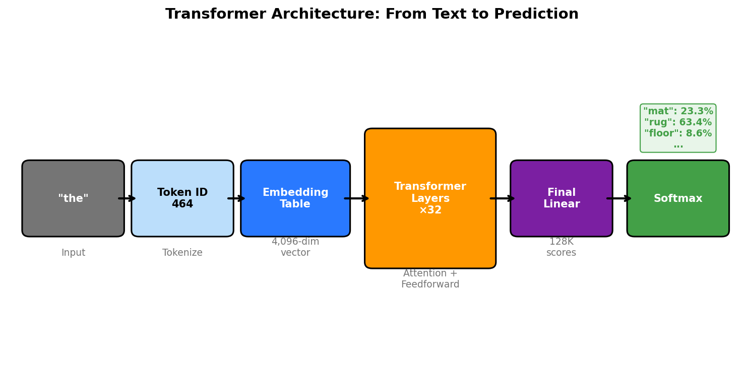
Large language models generate text one token at a time. A token is roughly a word or a piece of a word. “cat” is one token. “understanding” might get split into “under” and “standing” as two tokens. The model’s vocabulary is a fixed list of these tokens, typically 32,000 to 128,000 entries.

Internally, the model does not work with words as text. It converts each token into a list of numbers called an embedding. This is a vector, a point in a high-dimensional space. For example, the token “cat” might become a vector of 4096 numbers:

"cat" → [0.12, -0.34, 0.56, 0.01, ..., -0.23]   (4096 numbers)

Why 4096? That is a design choice. It is the hidden dimension of the model, sometimes called d_model. Larger models use more dimensions. GPT-2 uses 768. Llama-3.1-8B uses 4096. Llama-3.1-70B uses 8192. More dimensions means the model can encode more nuance about each token, but it also means more memory and computation.

How does a word get its embedding values? Before training, every token’s embedding is just random numbers. “cat” might start as [0.52, -0.11, 0.87, …] and “dog” might start as [0.33, 0.76, -0.44, …], completely meaningless. During training, the model reads billions of sentences and gradually adjusts these numbers. Tokens that appear in similar contexts (like “cat” and “kitten”, which both appear near words like “pet”, “fur”, “purred”) get their embeddings pushed closer together. Tokens that appear in very different contexts (like “cat” and “spreadsheet”) get pushed apart. How exactly the model learns these relationships during training is outside the scope of this article. I may cover that in a subsequent post.

After training, the embedding values encode patterns the model learned. But no single dimension has a clean human-readable meaning like “dimension 7 measures how alive something is.” It is more like mixing paint: no individual drop of color means “sunset,” but the right combination of many colors produces it. The model spreads meaning across all 4096 dimensions in whatever combination helps it predict text best.

What is the relationship between dimensions and parameters? The embedding table is itself a big grid of learned numbers. If the model has a vocabulary of 128,000 tokens and each embedding has 4096 dimensions, the embedding table alone contains 128,000 × 4096 = roughly 524 million numbers. Each of these numbers is a parameter, a value the model learned during training. On top of the embedding table, the model has many weight matrices, which are grids of learned numbers that transform the embeddings as they pass through the model. I will explain what W_Q, W_K, W_V, feed-forward networks, and layers are in the sections below. For now, the point is that the model has many such matrices and they are all filled with learned parameters. Add everything up and you get 8 billion parameters for Llama-3.1-8B.

So the dimension (4096) determines the shape of each matrix. The parameter count (8 billion) is the total number of learned values across all matrices in the model. A larger dimension means each token gets a richer representation but also means every matrix in the model gets bigger, which is why larger models have more parameters.

The embedding values tend to be small numbers, roughly between -1 and 1. The embedding values are learned during training. They start as random numbers and get adjusted as the model trains. They end up in a range where the math works well for the operations that follow. The exact values do not mean anything to a human, but the model learns that tokens with similar meanings end up with similar vectors. “cat” and “kitten” will have vectors that point in roughly the same direction, while “cat” and “spreadsheet” will point in very different directions.

Attention: How the Model Looks Back

Large language models generate text one token at a time. To decide what the next token should be, the model needs to look at all the tokens that came before it. This “looking back” is called attention. The mechanism was introduced in the paper “Attention Is All You Need” (Vaswani et al., 2017), which is the foundation of every modern transformer model.

Imagine you are writing a sentence and you have gotten to “The cat sat on the ___”. To fill in the blank, you need to look back at what you already wrote. Some previous words matter more than others. “cat” and “sat” are more relevant to your next word than “the”. Attention is how the model does this: it assigns a relevance score to every previous token and then pulls information from the most relevant ones.

Query, Key, and Value

For each token, the model computes three vectors. These are called the query, the key, and the value. The names come from database terminology, and the analogy is useful.

Think of a library catalog system:

• You walk in with a query: “I want books about animals”
• Every book on the shelf has an index card, a key: “this book is about cats”, “this book is about tax law”, “this book is about dogs”
• You compare your query against each key and find the best matches
• Each book also has actual content, the value: the pages inside the book
• You read the content (values) of the books whose keys matched your query

In the model, it works the same way:

"The cat sat on the ___"

Current position creates a query:   "what should come after 'the'?"
                                     query = [0.4, 0.6, 0.3]

Each previous token has a key:       "cat" key = [0.8, 0.3, 0.1]
                                     "sat" key = [0.5, 0.7, 0.2]
                                     ...

Each previous token has a value:     "cat" value = [0.1, 0.9, 0.4]
                                     "sat" value = [0.3, 0.5, 0.8]
                                     ...

These are not real numbers. I am using 3 dimensions to keep the examples readable. In an actual model like Llama-3.1-8B, each of these vectors has 128 dimensions. I will explain where that number comes from shortly.

Where do Q, K, V come from? They are computed by multiplying the token’s embedding by three separate weight matrices. A weight matrix is just a grid of numbers that the model learned during training. It transforms the embedding into a different representation suited for a specific purpose.

token embedding = [0.12, -0.34, 0.56, ...]   (4096 numbers)

query  = embedding × W_Q    (W_Q is a 4096 × 128 matrix of learned weights)
key    = embedding × W_K    (W_K is a 4096 × 128 matrix of learned weights)
value  = embedding × W_V    (W_V is a 4096 × 128 matrix of learned weights)

The multiplication squeezes the 4096-dimensional embedding down to 128 dimensions. Each weight matrix extracts different information from the embedding. W_Q extracts “what am I looking for?”, W_K extracts “what do I contain?”, and W_V extracts “what information do I carry?” The model learns these matrices during training. After training, they are fixed.

The Attention Calculation Step by Step

Say the model has generated “The cat sat on the” and is deciding the next token. Here is a worked example with 3 dimensions.

Step 1: Compare the query against every key using a dot product.

A dot product is a way to measure how similar two vectors are. You multiply corresponding elements and add them up. Two vectors pointing in the same direction give a high dot product. Two vectors pointing in different directions give a low one.

Query for next token: [0.4, 0.6, 0.3]

query · "The" key:  0.4×0.2 + 0.6×0.1 + 0.3×0.4 = 0.26
query · "cat" key:  0.4×0.8 + 0.6×0.3 + 0.3×0.1 = 0.53
query · "sat" key:  0.4×0.5 + 0.6×0.7 + 0.3×0.2 = 0.68
query · "on"  key:  0.4×0.1 + 0.6×0.9 + 0.3×0.4 = 0.70
query · "the" key:  0.4×0.3 + 0.6×0.1 + 0.3×0.5 = 0.33

“on” (0.70) and “sat” (0.68) score highest. “The” (0.26) scores lowest. This means the model considers “on” and “sat” most relevant for predicting what comes next.

Step 2: Convert scores to probabilities using softmax.

The raw dot products are just numbers. The model normalizes them into probabilities that add up to 1 using a function called softmax (it exaggerates the differences and makes them sum to 1).

Raw scores:    [0.26, 0.53, 0.68, 0.70, 0.33]
After softmax: [0.11, 0.18, 0.21, 0.22, 0.13]   (these add up to ~1.0)
                 The   cat   sat   on    the

Step 3: Use the probabilities to take a weighted average of the values.

Now the model multiplies each token’s value vector by its attention probability and adds them all up. Tokens with higher attention scores contribute more.

Output = 0.11 × value("The") + 0.18 × value("cat") + 0.21 × value("sat")
       + 0.22 × value("on")  + 0.13 × value("the")

       = 0.11 × [0.7, 0.3, 0.1] + 0.18 × [0.1, 0.9, 0.4] + 0.21 × [0.3, 0.5, 0.8]
       + 0.22 × [0.6, 0.2, 0.7] + 0.13 × [0.8, 0.4, 0.2]

       = [0.44, 0.44, 0.49]

This output vector is a blend of information from all previous tokens, weighted by relevance. The model feeds this into further layers to predict the next token (probably “mat” or “floor”).

One might wonder why we need both keys and values instead of just one vector per token. The reason is that matching and carrying information are different jobs. Consider a search engine: you search by keywords (keys) but what you read is the page content (values). If the key and the value were the same thing, the model would be forced to use the same representation for “is this token relevant?” and “what information does this token contribute?”, which is a much harder problem.

Attention Heads: Why Multiple Perspectives Help

I said that each query/key/value vector is 128 dimensions while the embedding is 4096. This is because the model does not run attention once. It runs it 32 times in parallel, each time with a different set of weight matrices. Each of these parallel runs is called an attention head.

Why? Because different words matter for different reasons. Consider “The cat that I adopted from the shelter last week sat on the ___”:

• One head might focus on the subject-verb relationship: “cat” … “sat” → what did the cat sit on?
• Another head might focus on recency: “week” → is the time reference relevant?
• Another might track the article-noun pattern: “the ___” → expects a noun

Each head gets its own 128-dimensional slice of the 4096-dimensional space:

Head 1: dims 0-127     → learns to track subject-verb patterns
Head 2: dims 128-255   → learns to track positional relationships
Head 3: dims 256-383   → learns to track adjective-noun patterns
...
Head 32: dims 3968-4095 → learns something else

Total: 32 heads × 128 dims = 4096 dims

(The labels like “subject-verb patterns” are just illustrative. The model learns what each head specializes in during training, and the actual patterns are usually more abstract than human-readable categories.)

Each head independently computes its own query, key, and value, runs the attention calculation, and produces its own 128-dimensional output. The 32 outputs are concatenated back into a 4096-dimensional vector. This is the mechanism described in the original transformer paper (Vaswani et al., 2017, Section 3.2.2).

Grouped Query Attention: a memory optimization. In the original transformer (Vaswani et al., 2017), every head has its own query, key, and value matrices. With 32 heads, that means 32 sets of keys and 32 sets of values stored in the cache for every token. Each key and value is 128 dimensions, so for one token at one layer, the KV cache stores 32 × 128 × 2 (keys + values) = 8,192 numbers.

Llama-3.1-8B uses a technique called Grouped Query Attention (GQA), introduced by Ainslie et al. (2023). The idea is that the 32 query heads do not all need their own private key-value pair. Instead, groups of 4 query heads share the same key and value.

This might seem wrong at first. If one query head focuses on syntax and another on topic, how can they share the same key? The key for the token “cat” is the same 128 numbers regardless of which query head is looking at it. But different query heads extract different information from the same key.

An analogy: think of a person’s resume. One interviewer is hiring for programming skills and reads the resume focusing on the technical experience section. Another interviewer is hiring for leadership and reads the same resume focusing on management experience. The resume is the same document (the shared key), but each interviewer (query head) picks up on different parts of it because they are looking for different things.

Same key vector for token "cat": [0.8, 0.3, 0.1, 0.7, 0.2, ...]
                                     ↑              ↑
                          dims 0-63 might encode     dims 64-127 might encode
                          syntactic role              semantic meaning

Query head A (tracking syntax):
  query_A · key = focuses on dims 0-63   → high score if "cat" is a subject

Query head B (tracking meaning):
  query_B · key = focuses on dims 64-127 → high score if "cat" is an animal

Same key, different scores, because the queries emphasize different dimensions.

In practice, the split is not as clean as “first half = syntax, second half = meaning.” The 128 dimensions encode many overlapping aspects simultaneously, and each query head learns during training which dimensions to pay attention to. The empirical result from the GQA paper is that sharing keys and values across 4 query heads causes almost no quality loss. 128 dimensions is rich enough that multiple query heads can each find what they need from the same key.

Original (32 query heads, 32 KV heads):
  Query head 1  → KV head 1
  Query head 2  → KV head 2
  ...
  Query head 32 → KV head 32

  KV cache per token per layer: 32 keys + 32 values = 64 vectors

Grouped Query Attention (32 query heads, 8 KV heads):
  Query heads 1-4   → share KV head 1
  Query heads 5-8   → share KV head 2
  ...
  Query heads 29-32 → share KV head 8

  KV cache per token per layer: 8 keys + 8 values = 16 vectors

Why the Cache Grows and Why It Hurts

When the model generates “mat” as the next token, it computes a new key and value for “mat” and appends them to the cache. Now there are 6 key-value pairs stored. For the token after “mat”, the model will compare against all 6. The cache keeps growing.

But the attention calculation I described above is not the whole story. The model does not run attention once and produce the output. It runs the token through a stack of identical processing blocks called layers, one after another. Each layer takes the output of the previous layer, runs its own attention (with its own separate weight matrices and its own separate attention heads), and then applies a feed-forward network to further transform the result.

Think of it like an assembly line. The first layer might pick up on surface-level patterns (“the” is usually followed by a noun). The second layer builds on that (“the cat” is a noun phrase that is the subject of the sentence). By layer 10 or 15, the model is working with abstract representations of meaning. By the final layer, it has enough context to predict the next token.

Llama-3.1-8B has 32 of these layers. The number 32 is a design choice made by Meta when they built the model. There is no universal rule that says “use 32 layers.” Smaller models use fewer layers (GPT-2 Small has 12 layers), larger models use more (Llama-3.1-70B has 80 layers). More layers means the model can learn more complex patterns, but it also means more computation and more memory. The specific numbers (32 layers, 32 query heads, 8 KV heads, 128 dimensions per head) are all choices that Meta made to balance quality against cost for an 8-billion-parameter model.

Each layer has its own complete set of attention heads with its own weight matrices. The keys and values produced by layer 1 are completely separate from those produced by layer 2. To see the scale, here is what happens when a single token “cat” passes through the model:

Token "cat" passes through 32 layers:

Layer 1:  32 query heads (128 dims each), 8 KV heads (128 dims each)
          → stores 8 key vectors + 8 value vectors in cache

Layer 2:  32 query heads (128 dims each), 8 KV heads (128 dims each)
          → stores 8 key vectors + 8 value vectors in cache

...

Layer 32: 32 query heads (128 dims each), 8 KV heads (128 dims each)
          → stores 8 key vectors + 8 value vectors in cache

Total KV cache for one token:
  32 layers × 8 KV heads × 128 dims × 2 (keys + values)
  = 32 × 8 × 128 × 2
  = 65,536 numbers stored per token

That is 65,536 numbers stored for a single token. For a 128K context window (131,072 tokens), multiply that out and you get the billions of numbers that make up the KV cache.

The memory cost scales as:

KV cache memory = 2 * num_layers * num_heads * head_dim * seq_len * bytes_per_value

2       → one set for keys, one for values
32      → layers
8       → KV heads per layer
128     → dimensions per head
131072  → sequence length (128K tokens)
2       → bytes per value (FP16 = 16 bits = 2 bytes)

For Llama-3.1-8B with a 128K context window:

2 * 32 * 8 * 128 * 131072 * 2 bytes = ~16 GB

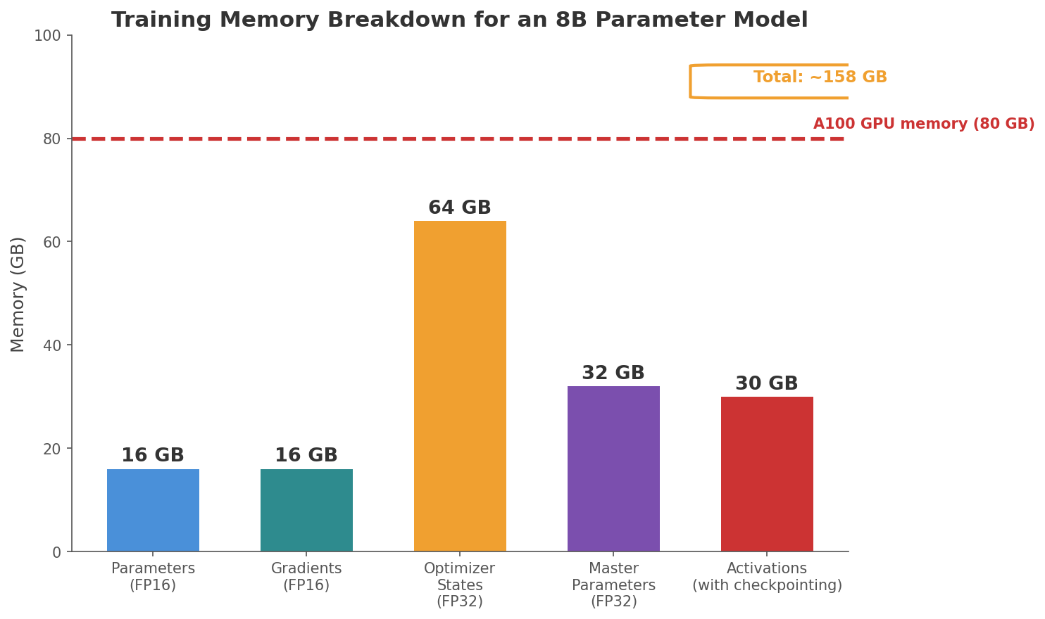
To put that in perspective, the model weights (all the learned parameters we discussed earlier, the embedding table, W_Q, W_K, W_V matrices, feed-forward networks across all 32 layers) are a fixed cost. The model has 8 billion parameters. Each parameter is stored in FP16 (2 bytes), so the model size is:

Model size = 8,000,000,000 × 2 bytes = 16 GB   (fixed, does not change)

The KV cache, on the other hand, depends on how long the conversation is:

Short conversation (1K tokens):
  2 × 32 × 8 × 128 × 1,024 × 2 bytes = ~128 MB     (small)

Medium conversation (16K tokens):
  2 × 32 × 8 × 128 × 16,384 × 2 bytes = ~2 GB       (noticeable)

Maximum context (128K tokens):
  2 × 32 × 8 × 128 × 131,072 × 2 bytes = ~16 GB     (as large as the model itself)

For a short chat, the KV cache is tiny compared to the model. But as the conversation gets longer, the KV cache grows while the model stays the same size. At maximum context length, they are roughly equal.

The real problem appears in batched serving, where you serve multiple users at the same time. The model weights are loaded once and shared across all users. But each user gets their own separate KV cache because each user has a different conversation. If you are serving 8 users with long contexts simultaneously:

Model weights:  16 GB   (shared, loaded once)
KV caches:      8 users × 16 GB = 128 GB   (separate per user)
Total:          144 GB

The KV cache is 8x larger than the model itself.

A smaller model has a smaller fixed cost but the KV cache scaling problem is the same. For Llama-3.1-70B (70 billion parameters, 80 layers, more heads), the model is larger but the KV cache also grows proportionally, and batched serving makes it worse.

When you see “200K context window” in Claude or “1M context” in Gemini, that number is the maximum number of tokens the model can look back at. It is the maximum length of the KV cache. The longer the context window, the more memory the KV cache consumes. This is why long-context models are expensive to serve and why there is so much interest in compressing the KV cache.

Quantizing the KV cache from FP16 (16 bits) down to 3 or 4 bits per value shrinks it by 4-5x. For the 8-user example above, that takes the KV cache from 128 GB down to around 25-30 GB, which is the difference between fitting on a single GPU and needing a whole cluster of them.

The Theory: How Much Can You Compress?

Shannon’s Rate-Distortion Function

Before looking at any specific algorithm, it helps to know the theoretical limit. How much can you compress something before the quality becomes unacceptable?

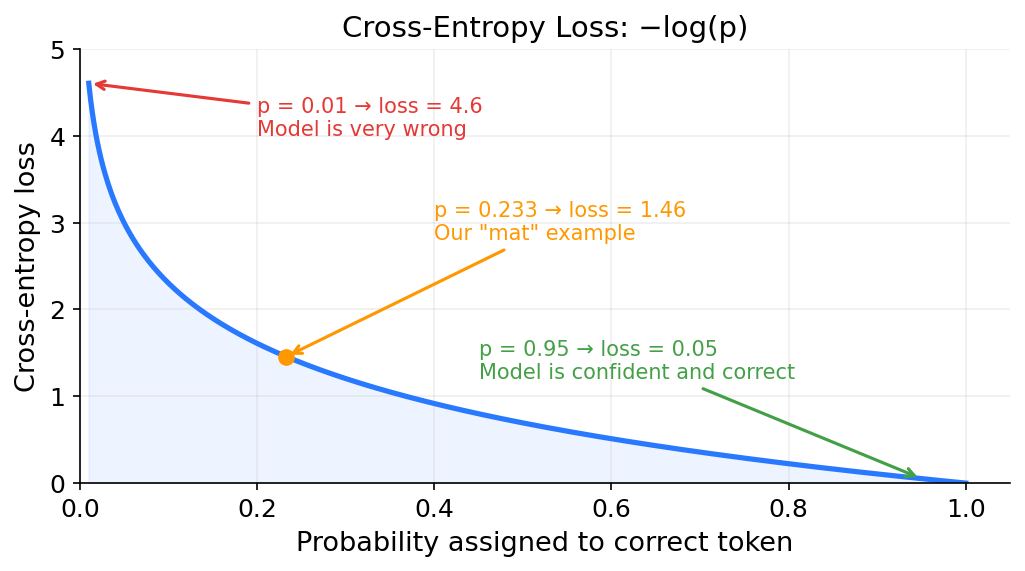
This is exactly the question Claude Shannon answered in his 1948 paper “A Mathematical Theory of Communication.” He introduced the rate-distortion function, which tells you the minimum number of bits per sample needed to keep the reconstruction error below some threshold.

To understand the formula, I need to explain a few terms.

Distortion is the error introduced by compression. If you store the number 0.87 but after compression and decompression you get back 0.85, the error is 0.02. The standard way to measure this across many values is mean-squared error (MSE): you take the difference between each original and reconstructed value, square it, and average over all values. Squaring makes large errors count more than small ones.

Variance (σ²) measures how spread out the data is. If all your values are close to the average, variance is low and the data is easier to compress (it is more predictable). If the values are spread all over the place, variance is high and you need more bits to capture the differences. The KV cache values in a transformer have some variance that depends on the model and the input.

Neural network activations are the intermediate values that flow through the model as it processes input. When a token passes through a layer, the attention mechanism and the feed-forward network produce output values at each step. These intermediate outputs are the activations. The key and value vectors in the KV cache are activations: they are computed on the fly as the model processes each token, not learned during training like the weights.

Gaussian source means the data follows a bell curve distribution. Most values cluster around the average, and values further from the average become increasingly rare.

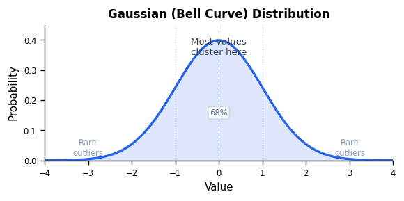
This is the most common assumption in information theory because many natural processes produce data that is approximately Gaussian. Neural network activations roughly follow this pattern too: most KV cache values are moderate, clustered around zero, with values further from zero becoming less common.

The assumption is not perfect though. In a true Gaussian distribution, extreme values (say, 100x larger than the average) are so rare that they essentially never happen. In real neural network activations, extreme values show up more often than a Gaussian would predict. These are the “outliers” we will see later when discussing SmoothQuant and KIVI. For example, in a layer’s activations, 99% of the values might be between -1 and 1, but a handful of channels consistently produce values of 50 or 100. This is what “heavier tails” means: the tails of the distribution (the extreme ends) have more probability mass than a Gaussian predicts.

Gaussian prediction:     value of 50 should appear 1 in 10^500 times  (never)
Real activations:        value of 50 appears in a few channels regularly

     Gaussian                     Real activations
       ╱╲                              ╱╲
      ╱  ╲                            ╱  ╲
     ╱    ╲                          ╱    ╲
    ╱      ╲                        ╱      ╲____
   ╱        ╲___                   ╱             ╲___
  ─────────────────               ──────────────────────
  tails drop fast                 tails drop slower (heavier)

Despite this mismatch, the Gaussian assumption is close enough for the theoretical analysis. Shannon’s rate-distortion formula gives a useful lower bound on how much you can compress, even if the real distribution is not exactly Gaussian. The practical quantization methods covered later in this article are designed to handle the outliers that the theory does not account for.

With those definitions, Shannon’s rate-distortion function for a Gaussian source is:

R(D) = (1/2) * log₂(σ² / D)

R(D)  = minimum bits per value needed
σ²    = variance of the data (how spread out the values are)
D     = maximum acceptable mean-squared error
log₂  = logarithm base 2 (because we are counting bits)

A concrete example: suppose the KV cache values have a variance of 1.0 (meaning the values are spread out with a standard deviation of 1, so most values fall between -1 and 1) and you can tolerate a mean-squared error of 0.01.

R(0.01) = (1/2) * log₂(1.0 / 0.01)
        = (1/2) * log₂(100)
        = (1/2) * 6.64
        = 3.32 bits per value

This says no algorithm can represent these values with less than 3.32 bits per value while keeping the MSE at or below 0.01. It does not matter how clever your algorithm is. This is a hard mathematical floor. No compression algorithm can do better than this regardless of how clever it is.

If you want less distortion (say D = 0.001), you need more bits:

R(0.001) = (1/2) * log₂(1.0 / 0.001)
         = (1/2) * log₂(1000)
         = (1/2) * 9.97
         = 4.98 bits per value

And if you can tolerate more distortion (D = 0.1), you need fewer bits:

R(0.1) = (1/2) * log₂(1.0 / 0.1)
       = (1/2) * log₂(10)
       = (1/2) * 3.32
       = 1.66 bits per value

This is the fundamental tradeoff: fewer bits means more distortion, and Shannon tells you exactly where the floor is.

TurboQuant proves that for a given bit budget, its distortion is at most 2.7 times the minimum possible distortion from Shannon’s formula. To put that concretely: if Shannon’s bound says the minimum achievable MSE at 3 bits is 0.01, TurboQuant guarantees its MSE will be at most 0.027.

Most quantization algorithms in this space have no proven worst-case guarantee. They are tuned empirically and could degrade unpredictably on different data. TurboQuant’s bound means the distortion is predictable and bounded no matter what input it sees.

Why Quantize at All?

The KV cache stores values in FP16, which uses 16 bits per number. That gives very high precision but consumes a lot of memory, as we saw above. Quantization reduces the number of bits used to represent each value.

What do we gain? Memory savings. Storing each value in 4 bits instead of 16 bits cuts memory by 4x. For the 8-user serving example, that takes the KV cache from 128 GB down to 32 GB.

What do we lose? Precision. With 16 bits you can represent 65,536 distinct values. With 4 bits you only get 16. Every original value has to be rounded to one of those 16 levels, and that rounding introduces error. The question is how to do this rounding in a way that minimizes the error for a given bit budget.

There are two main approaches: scalar quantization and vector quantization.

Scalar Quantization

The simplest approach. You take each number independently and snap it to the nearest value in a fixed set of levels. If you have 4 bits, you get 2⁴ = 16 levels spread across the range of your data.

Scalar quantization (4-bit, 16 levels):

Fixed set of 16 levels (evenly spaced from 0.0 to 1.0):
  [0.0, 0.07, 0.13, 0.20, 0.27, 0.33, 0.40, 0.47,
   0.53, 0.60, 0.67, 0.73, 0.80, 0.87, 0.93, 1.00]

Each original value gets mapped to the closest level in this set:

  0.31 → 0.33  (closest level)
  0.87 → 0.87  (exact match)
  0.52 → 0.53  (closest level)
  0.14 → 0.13  (closest level)

Original values:   [0.31, 0.87, 0.52, 0.14]
Quantized values:  [0.33, 0.87, 0.53, 0.13]

Each value is stored as a 4-bit index (0-15) into the set of 16 levels.
4 values × 4 bits = 16 bits total.
Original was 4 values × 16 bits = 64 bits. That is a 4x compression.

Scalar quantization is simple, fast, and has good hardware support. The downside is that it treats every number in isolation. It does not know or care that the numbers might be related to each other.

Vector Quantization

Instead of quantizing each number on its own, vector quantization treats a group of numbers as a single point and maps the whole group to the nearest entry in a precomputed table. This table is called a codebook, and each entry in it is called a codeword. The codebook is like a palette of allowed colors: every input vector gets matched to the closest color in the palette.

Vector quantization (2D, 4 codewords):

Original vector: (0.31, 0.87)    ← this is a point in 2D space

Codebook (our palette of 4 allowed points):
  c0 = (0.25, 0.75)
  c1 = (0.75, 0.75)
  c2 = (0.25, 0.25)
  c3 = (0.75, 0.25)

Nearest codeword: c0 = (0.25, 0.75)
Encoded as: index 0

We have 4 codewords, so we need 2 bits to pick one of them
(00 = c0, 01 = c1, 10 = c2, 11 = c3). Those 2 bits encode the
entire pair of numbers at once, so on average that is 1 bit per number.

But this is not the full cost. The codebook itself also takes up
memory. In this example, the codebook has 4 codewords, each
containing 2 floats at 16 bits each, so the codebook costs
4 × 2 × 16 = 128 bits. That is real overhead. The key difference
is that the codebook is stored once and shared across all vectors.
If you are quantizing 10,000 vectors, the codebook cost is 128 bits
shared over 10,000 vectors, which adds about 0.01 bits per vector.
The more vectors you quantize, the more negligible this becomes.

So the true per-vector cost of VQ is: 2 bits (index) + a tiny
amortized share of the codebook.

The advantage of vector quantization is that it can adapt to the shape of the data. Imagine plotting thousands of 2D data points on a scatter chart. They will not be spread evenly across the entire square. They will cluster in certain regions. Scalar quantization ignores these clusters and uses a uniform grid everywhere, wasting levels on empty regions. Vector quantization can place its codewords right where the data actually is, putting more codewords in dense regions and fewer in empty ones.

To put it concretely: if your KV cache values tend to come in patterns (say, when dimension 3 is high, dimension 7 is usually also high), scalar quantization ignores that pattern and quantizes both dimensions independently. Vector quantization can learn a codeword that captures the pattern directly, representing both dimensions together with fewer bits and less error.

The tradeoff is complexity. Vector quantization needs a codebook, which has to be built from the data ahead of time using algorithms like Lloyd’s (covered in the next section). The encoding step requires finding the nearest codeword in the codebook, which is more expensive than just rounding a number. And decoding requires a table lookup instead of simple arithmetic. But at low bit rates (2-4 bits per value), the quality advantage over scalar quantization is real and grows as you compress more aggressively. This is the regime TurboQuant operates in.

Lloyd’s Algorithm (1957)

Lloyd’s algorithm is the classic method for building VQ codebooks. It is essentially k-means clustering applied to the quantization problem:

1. Start with an initial set of codewords
2. Assign each data point to the nearest codeword
3. Update each codeword to be the centroid of its assigned points
4. Repeat until convergence

One practical problem with Lloyd’s algorithm is: how do you pick the initial codewords? If you start with bad initial positions, the algorithm can converge to a poor solution. The Linde-Buzo-Gray (LBG) algorithm from 1980 solves this by starting with just one codeword (the average of all data points) and then repeatedly splitting each codeword into two, running Lloyd’s algorithm after each split. You go from 1 codeword to 2, then 4, then 8, and so on until you reach the desired codebook size. Each split doubles the codebook and each round of Lloyd’s refines the positions. This gives a more reliable initialization than picking random starting points.

The deeper problem with Lloyd’s algorithm for KV cache compression is that it needs all the data upfront. You have to pass over all your data points multiple times (steps 2-4 repeat until convergence) to build the codebook. This works fine for weight quantization, where the weights are fixed and you can spend as long as you want building the codebook offline.

But the KV cache is not fixed. It grows in real time. During autoregressive generation, which is how language models produce text, the model generates one token at a time. It produces “The”, then uses that to produce “cat”, then uses “The cat” to produce “sat”, and so on. Each new token adds a new key-value pair to the cache. You cannot pause generation, collect all the key-value vectors, run Lloyd’s algorithm to build a codebook, and then start quantizing. The vectors arrive one at a time and need to be compressed immediately.

You need an online algorithm, one that can quantize each vector as it arrives without knowing what vectors will come next. This is the specific constraint that TurboQuant addresses.

The Landscape: How LLMs Are Quantized Today

Weight Quantization

Weight quantization compresses the model’s learned parameters, the W_Q, W_K, W_V matrices and feed-forward network weights we saw earlier. A model like Llama-3.1-8B has about 8 billion of these weight values. At full precision (FP16, 16 bits each), that is roughly 16 GB. At INT4 (4-bit integers, where each weight is stored as one of 16 possible levels), it drops to about 4 GB.

The key property of weights is that they are static. Once training is done, the weights do not change. This means you can spend hours analyzing the weights to figure out the best way to quantize them. You only pay this cost once, and then you serve the quantized model forever. This offline analysis is called post-training quantization (PTQ).

The three most widely used methods are:

GPTQ (Frantar et al., October 2022) tries to figure out which weights matter most. Not all weights affect the model’s output equally. Some weights, if rounded slightly wrong, cause large errors in the output. Others can be rounded aggressively with little impact. GPTQ measures this sensitivity using the Hessian, which is a mathematical tool that tells you how much the model’s loss function changes when you perturb each weight. Weights with high Hessian values are quantized more carefully. GPTQ processes one layer at a time and is the standard method for compressing models to INT4 (4 bits per weight).

AWQ (Lin et al., June 2023) approaches the same problem from a different angle. Instead of looking at the weights directly, it looks at the activations. Activations are the intermediate values that flow through the model when it processes input. When a token’s embedding gets multiplied by a weight matrix, the result is an activation. When that result passes through an attention layer and then a feed-forward layer, each step produces more activations. The model uses these activations during inference, which is the process of running the model to generate output (as opposed to training, where the model is learning its weights).

AWQ observes that a small fraction of activation channels carry much larger values than the rest. A channel is one dimension of the activation vector. If a 4096-dimensional activation vector consistently has a value of 50.0 in dimension 42 but values below 1.0 in dimension 43, then dimension 42 is an outlier channel. The weights connected to channel 42 are more important because errors in those weights get amplified by the large activation value. AWQ protects these critical weights by scaling them up before quantization so they get finer-grained levels. This improves on GPTQ at INT4.

SmoothQuant (Xiao et al., November 2022) targets INT8 (8 bits per value) for both weights and activations. Quantizing activations is harder than quantizing weights because activations have outliers.

A concrete example shows why outliers are a problem. Suppose a layer produces these activation values across 4 channels:

Activations: [0.5, 0.3, 0.1, 100.0]
                                 ↑
                           outlier channel

To quantize with INT8 (256 levels), you need to set the quantization range to cover the full spread. The range must go from 0 to 100 to include the outlier. That means each of the 256 levels covers a step of 100/256 ≈ 0.39.

Quantization range: 0 to 100, step size = 0.39

  0.5  → rounds to 0.39   (error: 0.11)
  0.3  → rounds to 0.39   (error: 0.09)
  0.1  → rounds to 0.00   (error: 0.10)
  100  → rounds to 100.0  (error: 0.00)

The three small values (0.5, 0.3, 0.1) are all crammed into the first
two levels. They become nearly indistinguishable. Most of the 256 levels
are wasted on the range 1-100 where there is only one value.

SmoothQuant fixes this by redistributing the difficulty between the activation and the weight. The idea is that in a transformer, the output of a layer is always activation × weight. If you divide the activation by some factor s and multiply the weight by the same factor s, the product stays exactly the same:

Original:         activation × weight = result
SmoothQuant:      (activation / s) × (weight × s) = same result

For the outlier channel, you pick a large scaling factor. For the normal channels, you pick a small one:

Before SmoothQuant:
  Activations: [0.5,  0.3,  0.1,  100.0]
  Weights:     [2.0,  1.5,  3.0,    0.5]

Scaling factors per channel: [1, 1, 1, 50]
  (large factor for the outlier channel)

After SmoothQuant:
  Activations: [0.5/1, 0.3/1, 0.1/1, 100/50] = [0.5, 0.3, 0.1, 2.0]
  Weights:     [2.0×1, 1.5×1, 3.0×1, 0.5×50] = [2.0, 1.5, 3.0, 25.0]

The activation is now smooth: all values between 0.1 and 2.0.
The weight got rougher: 25.0 in the last channel.
But the product for each channel is unchanged:
  0.5×2.0 = 1.0     (same as before: 0.5×2.0)
  0.3×1.5 = 0.45    (same as before: 0.3×1.5)
  0.1×3.0 = 0.30    (same as before: 0.1×3.0)
  2.0×25.0 = 50.0   (same as before: 100×0.5)

Now the activation range is 0.1 to 2.0 instead of 0.1 to 100. Quantizing this with 256 levels gives a step size of about 0.008, which is precise enough to distinguish 0.1, 0.3, and 0.5 from each other. The weight got rougher, but weights are static and can be quantized more carefully using methods like GPTQ.

All three are scalar methods. They quantize each weight or activation value independently. They all have mature support on NVIDIA GPUs through CUDA (NVIDIA’s programming framework for running computation on GPUs) and are widely deployed in production serving of models like Llama, Mistral, and others.

KV Cache Quantization

The KV cache is a different problem from weight quantization. Weights are fixed once training is done, so you can analyze them carefully offline. The KV cache is dynamic. It grows with every token the model generates, and the values have different statistical properties from weights.

KIVI (Liu et al., February 2024) proposes 2-bit quantization for the KV cache. Its key observation is that keys and values have different outlier patterns and should not be quantized the same way.

In the key vectors, the outliers tend to appear in the same channels across all tokens. No matter what token produced the key, channel 50 might always have a large value. This is a per-channel pattern.

In the value vectors, the outliers tend to appear in the same token across all channels. Token 200 might have large values in every channel while other tokens are mild. This is a per-token pattern.

Key outlier pattern (same channel, all tokens):
              ch1    ch2    ch50   ch100
  Token 1:    0.3    0.1    98.0    0.2
  Token 2:    0.5    0.4    95.0    0.1
  Token 3:    0.2    0.3    101.0   0.4
                             ↑
                      channel 50 is always large

Value outlier pattern (same token, all channels):
              ch1    ch2    ch50   ch100
  Token 1:    0.3    0.1    0.5    0.2
  Token 2:    0.5    0.4    0.3    0.1
  Token 200:  85.0   72.0   91.0   88.0   ← this entire token is an outlier
  Token 3:    0.2    0.3    0.4    0.4

KIVI uses this difference. For keys, it sets the quantization range per-channel: channel 50 gets its own min/max (say 90 to 105), while channel 1 gets a tighter range (0 to 1). This way the 4 levels of 2-bit quantization are spread appropriately for each channel. For values, it sets the range per-token: token 200 gets its own wide range while normal tokens get tight ranges.

This is what asymmetric quantization means here: keys and values are handled with different strategies that match their outlier patterns. The result is 2-bit precision with no fine-tuning needed.

KVQuant (Hooper et al., January 2024) pushes further, targeting sub-4-bit quantization to make 10-million-token context windows feasible. At that scale, even small per-value savings multiply into hundreds of gigabytes.

One technique KVQuant uses is non-uniform quantization levels. In the scalar quantization examples earlier, we spaced levels evenly across the range. But if most values cluster near zero with a few outliers far away, evenly spaced levels waste most of their resolution on empty space. Non-uniform quantization places levels closer together where values are common and further apart where they are rare.

Uniform levels (4-bit, 16 levels from -10 to 10):
  |----|----|----|----|----|----|----|----|----|----|----|----|----|----|----|
  -10       -5        0         5        10
  Most values are between -1 and 1, but only 2 of 16 levels fall there.

Non-uniform levels (4-bit, 16 levels, clustered near zero):
  |--|--|--|--|----|-------|------------|------------|-------|----|----|--|--|
  -10  -2 -1  0   1      3            6            8       9  10
  8 of 16 levels fall between -2 and 2, where most values actually are.

KVQuant computes where the data is dense by looking at the distribution of KV values across a calibration dataset (a set of representative inputs run through the model before deployment). The KV cache is dynamic during inference, but the statistical patterns of which ranges are dense tend to be consistent across inputs for a given model. KVQuant also applies a rotation to the key vectors before quantization to reduce outliers, similar in spirit to SmoothQuant’s approach of redistributing the difficulty.

GEAR (Kang et al., March 2024) takes a completely different approach. Instead of quantizing every value in the KV cache, it separates the cache into two parts. The first part is a low-rank approximation: a compressed version that captures the main patterns in the data using far fewer numbers, similar to how a blurry photo captures the general shapes but loses the fine details. The second part is a sparse residual: it stores only the entries where the low-rank approximation was far off (the outliers), at full precision. Everything else is discarded. The idea is that most of the KV cache is predictable and compressible, and only a few entries need to be stored accurately.

All three are scalar approaches. They quantize or compress individual values in the KV cache, possibly with different strategies per channel or per token, but they do not treat groups of values as vectors.

The Google Blog’s Proposal: Three Algorithms

The Google Research blog post describes TurboQuant as combining two earlier algorithms from the same group: QJL and PolarQuant. Each solves a different piece of the KV cache compression problem. TurboQuant brings them together into a unified method.

QJL: 1-Bit Quantization with Zero Overhead

The first paper is QJL (Zandieh, Daliri, Han, June 2024), which stands for Quantized Johnson-Lindenstrauss.

To understand the problem QJL solves, consider what happens when you quantize a block of values. You reduce each value to a few bits, but you also need to store some bookkeeping information alongside the quantized data. Specifically, you need a scale factor (how wide is the range of values?) and a zero point (where does the range start?). Without these two numbers, the receiver cannot reconstruct the original values from the quantized bits.

Example: quantizing [0.12, 0.87, 0.53, 0.31] to 2 bits per value

Step 1: Find the range.
  Min = 0.12, Max = 0.87

Step 2: Create 4 evenly spaced levels (2 bits = 2² = 4 possible levels).
  Level 0 = 0.12
  Level 1 = 0.37
  Level 2 = 0.62
  Level 3 = 0.87

Step 3: Map each original value to the nearest level.
  0.12 → Level 0 (0.12)   stored as bit code 00
  0.87 → Level 3 (0.87)   stored as bit code 11
  0.53 → Level 2 (0.62)   stored as bit code 10
  0.31 → Level 1 (0.37)   stored as bit code 01

Stored data: [00, 11, 10, 01]
  That is 4 values × 2 bits each = 8 bits total for the data.

But to decode these bits back into numbers, you also need to know
the scale and zero point:
  Scale factor: (0.87 - 0.12) / 3 = 0.25   (stored as FP16, 16 bits)
  Zero point: 0.12                            (stored as FP16, 16 bits)

To reconstruct: value = zero_point + bit_code × scale
  00 → 0.12 + 0 × 0.25 = 0.12
  11 → 0.12 + 3 × 0.25 = 0.87
  10 → 0.12 + 2 × 0.25 = 0.62
  01 → 0.12 + 1 × 0.25 = 0.37

Total storage: 8 bits (data) + 32 bits (scale + zero point) = 40 bits
Effective: 40 bits / 4 values = 10 bits per value, not 2.

For a small block, the metadata overhead can dominate. At low bit widths (1-2 bits per value), this overhead partly defeats the purpose of compressing in the first place.

QJL sidesteps this problem entirely. It uses a result from high-dimensional geometry called the Johnson-Lindenstrauss (JL) lemma. The idea behind JL is that if you take vectors in a high-dimensional space (say 4096 dimensions) and multiply them by a random matrix to project them down to fewer dimensions, the distances and angles between the vectors are approximately preserved. Two vectors that were similar before the projection will still be similar after it, and two vectors that were different will still be different.

QJL takes this one step further. After applying the random projection, it keeps only the sign of each resulting coordinate: positive becomes +1, negative becomes -1. That is 1 bit per coordinate. No scale factor, no zero point, nothing else to store. The entire representation is just a string of sign bits.

QJL compression of a key vector:

Original key: [0.31, -0.72, 0.15, -0.44, ...]   (128 FP16 values = 2048 bits)
                          |
              Multiply by random matrix R
                          |
Projected:    [0.08, -0.23, 0.41, -0.15, ...]
                          |
              Keep only the sign
                          |
Stored:       [+1, -1, +1, -1, ...]              (128 bits, no metadata)

But how do you compute attention with sign bits? Attention needs the dot product between a query and a key (as we saw earlier). QJL keeps the query at full precision and only compresses the cached keys. To estimate the dot product between a full-precision query and a 1-bit key, QJL uses a formula that multiplies the absolute value of each query coordinate by the sign of the corresponding key coordinate and averages the result.

The paper proves two things about this estimate. First, it is unbiased: on average, the estimate equals the true dot product. It does not systematically overestimate or underestimate. Second, the variance (how much the estimate fluctuates around the true value) decreases as you use more dimensions. Variance measures the spread of the estimate: low variance means the estimate is reliably close to the truth, high variance means it jumps around. With 128 dimensions, the estimate is reasonably stable.

For KV cache, this means keys can be stored at 1 bit per dimension with zero memory overhead from metadata. The tradeoff is that 1 bit is extreme compression and the estimate is noisier than higher-bit methods. That is where PolarQuant comes in.

PolarQuant: Polar Coordinates for Quantization

PolarQuant (Han, Kacham, Karbasi, Mirrokni, Zandieh, February 2025) takes a completely different approach. Instead of compressing the raw numbers directly, it first changes the way the vector is represented.

To understand this, consider two ways to describe a location. You can say “go 3 blocks East and 4 blocks North” or you can say “go 5 blocks at a 53-degree angle.” Both describe the same point, but they use different coordinate systems. The first is Cartesian coordinates (x, y), which is what we normally work with. The second is polar coordinates (radius, angle), which separates “how far” from “which direction.”

Cartesian: (3, 4)          "3 East, 4 North"
Polar:     (5, 53°)        "5 blocks at 53 degrees"

The radius is the distance: √(3² + 4²) = √25 = 5
The angle is: arctan(4/3) ≈ 53°

PolarQuant converts KV cache vectors from Cartesian to polar coordinates before quantizing them. The insight is that in many models, the direction of a KV vector (which way it points in the high-dimensional space) carries more information than its magnitude (how long it is). Two tokens with similar meanings will have KV vectors pointing in similar directions, even if their magnitudes differ. By separating direction from magnitude, you can allocate more bits to the direction (which matters more) and fewer to the magnitude (which varies less).

The conversion works recursively, pairing up coordinates at each level:

Input: 4-dimensional vector [3, 4, 1, 2]

Step 1: Group into pairs: (3, 4) and (1, 2)

Step 2: Convert each pair from Cartesian to polar:
        (3, 4) → radius = √(9+16) = 5.0,    angle = arctan(4/3) = 53°
        (1, 2) → radius = √(1+4)  = 2.24,   angle = arctan(2/1) = 63°

Step 3: Now we have two radii: (5.0, 2.24). Group them as a pair.

Step 4: Convert that pair to polar:
        (5.0, 2.24) → radius = √(25+5) = 5.48,  angle = arctan(2.24/5.0) = 24°

Result: one final radius (5.48) and three angles (53°, 63°, 24°)

The final radius is just the length of the original vector. The angles capture the direction. For a vector with d dimensions, you end up with 1 radius and d-1 angles.

The angles have a useful property: they always fall within a bounded range (0° to 360°, or equivalently 0 to 2π). This makes them easier to quantize than the original Cartesian coordinates, which can be any real number. When you know the range upfront, you can place your quantization levels evenly across it without worrying about outliers stretching the range.

Before the polar conversion, PolarQuant applies a preprocessing step: it multiplies the vector by a Hadamard matrix. A Hadamard matrix is a specific type of square matrix filled with +1 and -1 values, arranged so that the multiplication spreads the energy of the vector evenly across all coordinates. Without this step, a few coordinates might carry most of the information while the rest are near zero. That would waste quantization levels on the near-zero coordinates. After the Hadamard rotation, every coordinate carries a roughly equal share of the information, so quantization levels are used efficiently. This same trick appears in QuIP and QuIP#, two earlier vector quantization methods for LLM weights.

PolarQuant pipeline:

Input vector v (128 dimensions)
       |
   Multiply by Hadamard matrix (spreads energy evenly)
       |
   Rotated vector v' (all coordinates now carry similar energy)
       |
   Recursive polar conversion (pair, convert, pair, convert, ...)
       |
   1 radius + 127 angles
       |
   Quantize angles with optimal scalar quantizers
       |
   Store: quantized angles + radius

The paper shows that PolarQuant achieves near-lossless KV cache compression. On the “needle in a haystack” benchmark, which tests whether the model can find a specific piece of information buried in a very long context (a task that is extremely sensitive to KV cache quality), PolarQuant matches the uncompressed model.

TurboQuant: Putting It Together

TurboQuant (Zandieh, Daliri, Hadian, Mirrokni, April 2025) combines the ideas from QJL and PolarQuant into a single framework with provable guarantees on how much error it introduces. It is being presented at ICLR 2026.

The core problem TurboQuant solves is: how do you build a vector quantizer that works well without seeing the data ahead of time? Lloyd’s algorithm needs multiple passes over the data. PolarQuant’s polar conversion is data-oblivious but does not have provable optimality guarantees. TurboQuant achieves both: data-oblivious operation and provable near-optimality.

The algorithm has two stages.

Stage 1: Rotate and quantize

The first step is to multiply the input vector by a random orthogonal matrix. An orthogonal matrix is a square matrix with a special property: multiplying a vector by it rotates the vector in space without changing its length or any of the angles between vectors. Nothing is stretched or squashed, the vector just points in a new direction.

A simple 2D example makes this concrete. The matrix below is orthogonal (each row has length 1, and the two rows are perpendicular to each other):

Orthogonal matrix (a 45-degree rotation):

  R = [ 0.71  -0.71 ]     row 1: length = √(0.71² + 0.71²) = 1.0  ✓
      [ 0.71   0.71 ]     row 2: length = √(0.71² + 0.71²) = 1.0  ✓
                           row1 · row2 = 0.71×0.71 + (-0.71)×0.71 = 0  ✓ (perpendicular)

Multiplying:

  R × [1.0, 0.0] = [0.71×1.0 + (-0.71)×0.0,  0.71×1.0 + 0.71×0.0]
                  = [0.71, 0.71]

Original:  (1.0, 0.0)     length = √(1² + 0²) = 1.0
Rotated:   (0.71, 0.71)   length = √(0.71² + 0.71²) = 1.0   (same length)

The vector was pointing along the x-axis, and the orthogonal matrix rotated it to point diagonally. The length stayed at 1.0.

This raises an important question: if we rotate the vector, do we lose the meaning encoded in it? The answer is no, and this comes from a core property of linear algebra. Orthogonal rotations preserve three things:

1. Lengths of vectors (as shown above).
2. Distances between any two vectors. If “cat” and “kitten” were close together before rotation, they are still exactly the same distance apart after rotation.
3. Dot products between any two vectors. This is the critical one for attention. Recall that attention computes the dot product between query and key vectors to find which tokens are relevant. If dot_product(query, key_A) > dot_product(query, key_B) before rotation, the exact same ordering holds after rotation. No attention scores change.

Before rotation:
  query · key_A = 0.85   (token A is more relevant)
  query · key_B = 0.32   (token B is less relevant)

After rotating ALL vectors by the same orthogonal matrix R:
  (R × query) · (R × key_A) = 0.85   (same score, exactly)
  (R × query) · (R × key_B) = 0.32   (same score, exactly)

The rotation changes the coordinate system, not the relationships between vectors. Think of it like rotating a map: all the cities move to new pixel positions, but the distances between them do not change. North might now point to the right instead of up, but Paris is still the same distance from London.

The reason this matters for quantization is that you can rotate the vectors into a coordinate system where they are easier to quantize (energy spread evenly, coordinates in a predictable range), quantize in that rotated system, and then the dot products you compute with the quantized vectors are the same as if you had quantized in the original system. You get the benefits of the rotation without changing what the model computes.

In TurboQuant, the rotation is in 128 dimensions instead of 2, and the orthogonal matrix is chosen randomly. But the same principle applies: lengths, distances, and dot products are all preserved.

Why rotate? Consider a KV cache vector where most of the information is concentrated in a few dimensions:

Before rotation:  [5.2, 0.01, 0.03, 8.1, 0.02, 0.01, ...]
                    ↑                  ↑
              These two dimensions carry almost all the energy.
              The rest are near zero.

If you quantize this directly with, say, 4 levels per dimension, you waste 3 of the 4 levels on the near-zero dimensions (they are all roughly the same, so you do not need 4 levels to represent them). Meanwhile, the two important dimensions really need more than 4 levels.

After a random rotation, the energy gets spread evenly:

After rotation:   [1.4, 1.2, 0.9, 1.3, 1.1, 1.0, ...]
                   All dimensions now carry similar energy.
                   4 levels per dimension is used efficiently everywhere.

This is the same idea as the Hadamard rotation in PolarQuant, but TurboQuant uses a random orthogonal matrix instead of a fixed Hadamard matrix. The difference matters for the theory. A fixed matrix like Hadamard works well in practice, but an adversary could construct a specific input vector that is already aligned with the Hadamard matrix in a way that the rotation does not help. A random matrix does not have this weakness: because the matrix is chosen randomly, no input vector can be “pre-aligned” with it. This is what allows TurboQuant to prove worst-case guarantees that hold for any input, not just typical inputs. The TurboQuant paper (Theorem 1) formalizes this.

The rotation also has a second benefit that is specific to high-dimensional spaces. In 2 or 3 dimensions, a random rotation can move energy around in unpredictable ways. But in 128 dimensions, a mathematical result called the concentration of measure phenomenon kicks in. It says that after a random rotation, every single coordinate of the rotated vector ends up close to the same value. Not approximately, not usually, but with high probability. The higher the dimension, the tighter this concentration.

The distribution each coordinate follows is called a Beta distribution. Unlike the Gaussian (bell curve), which stretches from negative infinity to positive infinity, the Beta distribution lives within a fixed bounded range (between 0 and 1, after scaling). In 128 dimensions, the Beta distribution is very narrow: most coordinates end up clustered tightly around a single predictable value.

Before rotation (128 dims): values all over the place
  [5.2, 0.01, -3.1, 0.03, 8.1, -0.5, ...]   range: -3.1 to 8.1

After random rotation (128 dims): values concentrated
  [0.41, 0.38, 0.43, 0.39, 0.40, 0.42, ...]  range: roughly 0.35 to 0.45

Each coordinate independently follows a Beta distribution
centered around ≈ 0.40 with very little spread.

This concentration is what makes the whole approach work. Because the distribution is known and narrow, you can design quantization levels that are perfectly matched to it. No levels are wasted on values that will never appear.

Before rotation: coordinate values can be anything
                  [-8.1, 0.01, 5.2, -0.3, ...]  (unpredictable, wide range)

After rotation:   each coordinate ≈ Beta distributed
                  [0.41, 0.38, 0.43, 0.39, ...]  (predictable, narrow range)

Because this distribution is known in advance (it comes from the math of random rotations, not from the data), the optimal quantization levels for each coordinate can be computed once and reused forever. There is no codebook to learn, no Lloyd’s algorithm to run, no calibration data to collect. The quantizer is fully determined by two things: how many dimensions the vector has and how many bits you want to use per dimension.

This is what data-oblivious means: the quantization scheme is fixed before you see any data. A new token arrives, you rotate its key/value vector, quantize each coordinate using the precomputed levels, and you are done. No adaptation, no learning, no state to maintain. This is exactly what you need for the KV cache, where vectors arrive one token at a time during generation.

The paper proves that this approach achieves distortion within a factor of 2.7 of Shannon’s theoretical minimum. As we covered earlier, the fact that it can guarantee a constant factor bound at all is what matters: the distortion is predictable and bounded no matter what input it sees.

Stage 2: Fix the dot product error with QJL

Stage 1 does a good job of minimizing reconstruction error (the difference between the original vector and the quantized version). But reconstruction error is not what attention cares about. Attention computes the dot product between query and key vectors. It is possible for a quantizer to have low reconstruction error but still give bad dot product estimates.

Here is why. Suppose quantization consistently rounds values slightly upward. The reconstructed vector is close to the original (low MSE), but every dot product computed with it is slightly too high because both vectors got bumped up. This systematic shift is called bias.

Example of bias in dot products:

Original vectors:  a = [1.0, 2.0]     b = [3.0, 1.0]
True dot product:  1.0×3.0 + 2.0×1.0 = 5.0

Quantized (biased upward):
  a' = [1.1, 2.1]    b' = [3.1, 1.1]
  Estimated dot product: 1.1×3.1 + 2.1×1.1 = 3.41 + 2.31 = 5.72

The MSE is small (each value is off by 0.1), but the dot product
estimate is 5.72 instead of 5.0. That is a 14% error, which
could shift which tokens get the highest attention scores.

To fix this, TurboQuant adds a correction step using QJL. First, it computes the residual: the difference between the original vector and the quantized version. The residual captures everything the quantizer got wrong.

Original (after rotation):   v' = [0.41, 0.38, 0.43, 0.39, ...]
Quantized:                  q(v') = [0.40, 0.40, 0.45, 0.40, ...]
Residual:                   error = [0.01, -0.02, -0.02, -0.01, ...]

TurboQuant then applies the QJL transform to this residual. As we saw in the QJL section, this means: multiply by a random matrix, then keep only the sign of each result.

Residual:               [0.01, -0.02, -0.02, -0.01, ...]
                              |
              Multiply by random matrix R
                              |
Projected residual:     [0.003, -0.015, 0.008, -0.012, ...]
                              |
              Keep only the sign
                              |
Stored:                 [+1, -1, +1, -1, ...]    (1 bit each, no metadata)

This costs just 1 extra bit per dimension and adds zero metadata overhead.

At attention time, the dot product estimate combines the quantized vectors and the QJL correction. The QJL correction cancels out the bias from the quantizer, producing an unbiased estimate of the true dot product.

TurboQuant full pipeline:

Input vector v (128 dimensions, FP16 = 16 bits per dim)
       |
   Multiply by random orthogonal matrix R
       |
   v' = Rv  (each coordinate now Beta distributed, predictable range)
       |
   Quantize each coordinate using precomputed levels
       |
   q(v') stored in 3 bits per dimension
       |
   Compute residual: error = v' - q(v')
       |
   Apply QJL to residual → 1 sign bit per dimension
       |
   Total storage per dimension: 3 bits (quantized) + 1 bit (QJL) = 4 bits
   Compression: 16 bits → 4 bits = 4x reduction

At attention time:
   dot_product(query, key)
     ≈ dot_product(q(query'), q(key'))     ← from quantized vectors
       + QJL_correction(residual)           ← removes bias

The total cost per dimension is the quantization bits plus 1 bit for the QJL correction. At 3 bits of quantization plus 1 bit of QJL, that is 4 bits per dimension total, a 4x compression from FP16. At 2 bits of quantization plus 1 bit of QJL, that is 3 bits total, roughly a 5x compression.

Benchmark Results

The Google blog reports evaluations across standard long-context benchmarks (LongBench, Needle In A Haystack, ZeroSCROLLS, RULER, and L-Eval) using open-source models (Gemma and Mistral), with additional results on Llama-3.1-8B-Instruct for the LongBench benchmark.

KV cache compression quality: TurboQuant quantizes the KV cache to 3 bits without requiring training or fine-tuning and without any compromise in model accuracy. The blog frames this as achieving “optimal scoring performance in terms of both dot product distortion and recall while simultaneously minimizing the KV memory footprint.”

Needle-in-haystack tasks: These tests check if a model can find one specific, tiny piece of information buried inside a massive amount of text. TurboQuant achieves perfect scores across all benchmarks while reducing the KV memory by a factor of at least 6x. PolarQuant is also nearly lossless on this task. If the KV cache loses too much precision, the model forgets information from earlier in the context and either makes something up or gives a wrong answer.

Runtime performance: The blog describes TurboQuant as “exceptionally efficient to implement” with “negligible runtime overhead.” 4-bit TurboQuant achieves up to 8x speedup in computing the attention scores over the 32-bit (FP32) unquantized baseline. The comparison is against FP32, not FP16 which is the more common precision used in production inference. The speedup relative to FP16 would be roughly half (4x), since FP16 is already 2x smaller than FP32.

Vector search: Beyond KV cache compression, TurboQuant was also evaluated on high-dimensional vector search using the GloVe dataset (200 dimensions). It achieves better recall ratios than existing methods (Product Quantization and RabbiQ), despite those baselines using data-dependent training while TurboQuant is data-oblivious.

The blog highlights Gemini as a major application for this work and notes that the impact extends to semantic search at Google’s scale.

Sources

• Google Research Blog: TurboQuant: Redefining AI efficiency with extreme compression (March 2026)
• Shannon, C. E. (1948). A Mathematical Theory of Communication. Bell System Technical Journal
• Lloyd, S. P. (1982). Least Squares Quantization in PCM. IEEE Transactions on Information Theory
• Linde, Buzo, Gray (1980). An Algorithm for Vector Quantizer Design. IEEE Transactions on Communications
• GPTQ: Frantar et al. (2022). Accurate Post-Training Quantization for Generative Pre-trained Transformers
• AWQ: Lin et al. (2023). Activation-aware Weight Quantization for LLM Compression and Acceleration
• SmoothQuant: Xiao et al. (2022). Accurate and Efficient Post-Training Quantization for Large Language Models
• QuIP: Chee et al. (2023). 2-Bit Quantization of Large Language Models With Guarantees
• QuIP#: Tseng et al. (2024). Even Better LLM Quantization with Hadamard Incoherence and Lattice Codebooks
• AQLM: Egiazarian et al. (2024). Extreme Compression of Large Language Models via Additive Quantization
• QJL: Zandieh, Daliri, Han (2024). 1-Bit Quantized JL Transform for KV Cache Quantization with Zero Overhead
• KIVI: Liu et al. (2024). A Tuning-Free Asymmetric 2bit Quantization for KV Cache
• KVQuant: Hooper et al. (2024). Towards 10 Million Context Length LLM Inference with KV Cache Quantization
• GEAR: Kang et al. (2024). An Efficient KV Cache Compression Recipe for Near-Lossless Generative Inference of LLM
• PolarQuant: Han, Kacham, Karbasi, Mirrokni, Zandieh (2025). Quantizing KV Caches with Polar Transformation
• TurboQuant: Zandieh, Daliri, Hadian, Mirrokni (2025). Online Vector Quantization with Near-optimal Distortion Rate
• ECO: Nikdan et al. (2026). Quantized Training without Full-Precision Master Weights

Garbage Collection: From First Principles to Modern Collectors in Java, Go and Python

Over the last few years I have gone from Java to Go to Rust and now back to Java. The one thing that keeps coming up when switching between these languages is garbage collection. Java and Go have it, Rust does not. In benchmarks, in latency discussions, in “why is this service slow” conversations, GC is always somewhere in the picture. I kept hearing about GC pauses, throughput overhead and write barriers, but I did not completely understand what was happening underneath.

While looking for the origins I came across McCarthy’s 1960 paper, which is famous for introducing Lisp but also happens to be where mark-and-sweep was first described. That led me to Wilson’s 1992 survey, “Uniprocessor Garbage Collection Techniques”, which organizes everything that followed into a clean taxonomy. Reading both made the modern collectors much easier to understand, because G1GC, ZGC, Go’s concurrent collector and CPython’s hybrid approach are all variations on ideas those papers describe. I also wrote a toy GC in Go to see the mechanics for myself.

These are my notes from that process.

The Papers That Started It

McCarthy (1960): Recursive Functions of Symbolic Expressions and Their Computation by Machine

This paper is famous for introducing Lisp, but the garbage collector is buried in it almost as an implementation detail. McCarthy needed a way to manage memory for symbolic expressions. Lisp programs manipulate lists of lists of lists, and the recursive structure made it impractical to ask programmers to free memory manually. So he described a mechanism to do it automatically.

The mechanism is two phases. First, start from the root variables the program is actively using and traverse every object they reference, flagging each one as reachable. Second, scan all of memory. Anything not flagged is garbage. Add it back to the free list.

That is mark-and-sweep. It handles cycles naturally (unreachable cycles never get flagged), requires no per-object bookkeeping and lets the programmer ignore memory entirely.

The cost was that the program had to stop completely while the collector ran. Every allocation, every computation, everything froze until the mark and sweep finished. For the programs McCarthy was writing in 1960, this was perfectly reasonable. As programs grew larger and moved into latency-sensitive environments like web servers handling thousands of requests per second, stopping the world became a harder tradeoff to accept. Most of what modern GC research has produced is the answer to one question: how do you collect garbage without stopping the world?

Wilson (1992): Uniprocessor Garbage Collection Techniques

By 1992, thirty years of GC research had produced a lot of ideas but there wasn’t much of shared vocabulary. Wilson’s survey is the paper that organized it all. It is not a new algorithm. It is a taxonomy that gives names and structure to ideas that were scattered across decades of papers.

Wilson formalizes the three classic algorithms that everything else is built on.

The first is mark-and-sweep, which is McCarthy’s original algorithm. Start from the roots, walk the object graph, mark everything you can reach, then sweep through the heap and free anything unmarked. It handles cycles naturally and the implementation is straightforward. The downside is that after enough cycles of allocation and collection, the heap gets fragmented. Live objects end up scattered with small free gaps between them and the allocator has to search harder to find space.

The second is copying, sometimes called semi-space. The idea is to split the heap into two halves. You allocate in one half, and when it fills up, you copy all the live objects into the other half and throw the first one away entirely. Fragmentation disappears because live objects get packed together during the copy. Allocation is fast because you just bump a pointer forward. The cost is that half your memory is always sitting empty, waiting to be the destination for the next copy.

The third is reference counting. Every object keeps a count of how many pointers point to it. When a new reference is created, the count goes up. When a reference is removed, it goes down. When it hits zero, the object is freed immediately. There is no tracing, no pause and destruction is deterministic. The problem is cycles. If two objects point to each other, both have a count of at least 1, even when nothing else in the program can reach them. Neither will ever be freed by reference counting alone.

Beyond the three algorithms, Wilson explores two observations that modern collectors depend on.

The first is the generational hypothesis: most objects die young. In practice, the temporary objects a program allocates (intermediate values, request-scoped buffers, loop variables) tend to become garbage very quickly, while a small fraction of objects live for the entire program. If you collect young objects frequently and old objects rarely, you do most of your work on the part of the heap that is mostly garbage, which is much cheaper than scanning everything every time.

The second is tricolor marking, an abstraction for incremental and concurrent collection. Instead of marking objects as simply visited or unvisited, you use three colors: white (not yet seen), grey (seen but children not yet scanned), and black (fully processed). The collector processes grey objects one at a time. At termination, white objects are garbage. This abstraction is what makes it possible to run the collector and the application simultaneously without them corrupting each other’s view of the heap. Go’s concurrent mark-and-sweep and ZGC’s concurrent marking are both direct descendants of this idea.

Everything in the “Modern GCs” section of this article maps back to one of Wilson’s categories. The engineering has gotten much more sophisticated, but the underlying structure is the same.

The Two Fundamental Approaches

Almost every garbage collector is either reference counting, tracing or some combination of both. Wilson’s paper is organized around this split, and it still holds thirty years later.

Reference Counting

Each object maintains a count of how many references point to it. When a reference is created, the count goes up. When a reference is removed, it goes down. When it hits zero, the object is freed immediately.

Object A (refcount: 2)  <--- pointer from B
                         <--- pointer from C

C.ref = null   -->  Object A (refcount: 1)  // still alive
B.ref = null   -->  Object A (refcount: 0)  // freed immediately

This is what CPython uses as its primary mechanism. It is simple and gives you deterministic destruction. When the last reference to a file handle goes away, __del__ runs and the file closes right there, not at some later GC cycle.

Two problems make reference counting insufficient on its own.

Cycles. If Object A points to Object B and Object B points back to A, both maintain a count of at least 1 even when nothing else in the program can reach them. Neither is ever freed.

  Object A (refcount: 1) ---> Object B (refcount: 1)
       ^                           |
       |___________________________|

  Nothing else points to A or B.
  Both are garbage, but refcount never hits 0.

This is not a theoretical edge case. Cycles show up naturally in linked data structures, parent-child relationships, observer patterns and caches. I will talk about how Python deals with this when we get to CPython’s GC later in the article.

Per-mutation overhead. Every pointer assignment requires updating reference counts. In a multithreaded program these must be atomic operations, which are significantly more expensive. Every time you pass an object to a function, return it, or assign it to a field, you pay this cost.

Tracing (Mark-and-Sweep)

Instead of tracking individual references, a tracing collector starts from a set of known-live references called the root set and traverses the entire object graph. Every object it can reach gets marked as alive. Everything else gets freed.

The root set is the starting point, so the definition of what counts as a root matters. The answer is the same across languages: a root is any reference the runtime can find without tracing. These are the pointers anchored to the program’s execution stateright now, the things you know are alive before any traversal begins.

In practice, roots fall into a few categories.

Local variables and function arguments in every active stack frame are roots. The program is actively running those functions, so anything they reference is by definition in use.

Global and static variables are roots because they live for the entire lifetime of the program.

CPU registers are roots because when a JIT compiler optimizes a hot method, it may keep a frequently accessed object reference in a CPU register instead of writing it back to the stack. If the GC runs at that moment, the register holds the only live reference to that object. If the GC does not scan registers, it would free an object that is still in use. To prevent this, the runtime defines safe points in the code where GC can only occur, and at those points it snapshots the register state to find any references held there.

The runtime itself also holds roots that have nothing to do with user code. In the JVM, class loaders are roots: every class you load is referenced by its class loader, and as long as the class loader is alive, every class it loaded (including their static fields) stays alive. Interned strings are roots because String.intern() stores strings in a shared pool that the JVM maintains. JNI handles are roots because when native C or C++ code holds a reference to a Java object via the Java Native Interface, that reference lives outside the Java heap in a handle table that the GC must scan. Each live thread is a root, and its entire call stack of frames is part of the root set.

Go’s runtime follows the same principle. Each goroutine has its own stack, and all goroutine stacks must be scanned to find roots. The runtime also tracks its own internal data structures, such as the finalizer queue, as part of the root set.

Stack frame (main)              Stack frame (handleRequest)
  conn   ------------------>  [Connection object] --> [Buffer]
  config ------------------>  [Config object]
                                request  ---------> [Request object]
                                response ---------> [Response object]

Everything reachable from these stack variables is alive.
Anything else on the heap is garbage.

The key insight is that roots are defined by what the runtime already knows is live without tracing. Everything else must earn its survival by being reachable from a root. This is why the concept is language-agnostic. The specific set of roots differs between Java, Go and Python, but the principle is the same: start from what you know is live, trace outward and reclaim the rest.

Cycles are handled naturally. If A and B point to each other but neither is reachable from any root, the mark phase never visits them. They remain unmarked and get swept.

The cost: a naive mark-and-sweep must pause the entire program while it traces the heap. This stop-the-world pause was the defining problem of early garbage collectors and is what modern GCs have spent decades engineering around.

Why Most Modern GCs Are Tracing-Based

Reference counting’s per-mutation cost adds up in server workloads with high allocation rates. Every pointer write increments or decrements a count. In a multithreaded program those updates must be atomic, and atomic operations are expensive. At thousands of allocations per second across dozens of threads, that overhead becomes measurable. The cycle problem requires a supplementary tracing pass anyway. And tracing collectors can be made concurrent, running alongside the application with only brief pauses.

Java and Go use tracing collectors. Python is the notable exception. It starts with reference counting and layers a tracing cycle detector on top.

Tracing Variants

Wilson’s paper describes four ways to implement tracing, each with different tradeoffs.

Mark-Sweep

The simplest tracing collector. Two phases:

1. Mark: Starting from roots, traverse the object graph and set a mark bit on every reachable object.
2. Sweep: Walk through the entire heap. Any object without a mark bit is garbage. Free it and add the memory back to the free list.

Roots: [A, C]

Heap before marking:
  [A] --> [B] --> [D]
  [C] --> [E]
  [F]            (unreachable)
  [G] --> [H]    (unreachable)

After mark phase:
  [A*] --> [B*] --> [D*]     (* = marked/alive)
  [C*] --> [E*]
  [F]                         (not marked)
  [G] --> [H]                 (not marked)

Sweep phase: free F, G, H

The main problem with mark-sweep is fragmentation. After enough collection cycles, the heap looks like Swiss cheese: live objects scattered across it with small free gaps between them. You might have 100MB free in total but no single contiguous block large enough to satisfy a new allocation. The allocator has to maintain a free list and search it for a fit, which gets slower as the heap gets more fragmented.

Copying (Semi-Space)

The heap is divided into two equal halves: from-space and to-space. Allocation happens in from-space using a simple bump pointer. When from-space fills up, the collector copies all live objects into to-space, updates all pointers, then swaps the roles. The old from-space is discarded entirely.

From-space:  [A*][garbage][B*][garbage][C*]
To-space:    [empty........................]

After collection:
From-space:  [freed entirely................]
To-space:    [A*][B*][C*][free.............]

Allocation is extremely fast because it is just a pointer bump. Compaction happens naturally. The cost is that only half the heap is usable at any time.

Mark-Compact

Same marking phase as mark-sweep, but instead of just freeing unmarked objects, the collector slides all live objects to one end of the heap. This eliminates fragmentation without the 50% memory overhead of copying collectors.

Before compaction:
  [A*][___][B*][___][___][C*][___][D*]

After compaction:
  [A*][B*][C*][D*][___][___][___][___]
                   ^
                   free pointer (bump allocation from here)

The downside is that compaction requires multiple passes over the heap: one to mark, one to compute new addresses, one to update all pointers, one to move objects.

The Generational Hypothesis

One of the most influential observations in Wilson’s paper is the weak generational hypothesis: most objects die young.

In a typical web server, each request creates temporary objects (parsers, intermediate strings, response builders) that live for milliseconds. Configuration objects, connection pools and caches live for the entire application lifetime.

Generational collectors exploit this by dividing the heap into generations. New objects go into the young generation. If they survive a few collections, they get promoted to the old generation. Young generation collections are frequent and fast because most objects there are already dead. Old generation collections are rare.

+-------------------+---------------------+
|  Young Generation |   Old Generation    |
|  (collected often)|  (collected rarely) |
|                   |                     |
|  Eden | S0 | S1   |                     |
+-------------------+---------------------+

Eden is where all new objects are born. Every new Object() goes here. It fills up fast because most programs allocate at a high rate.

S0 and S1 are two small survivor spaces. When Eden fills up and a minor GC runs, the collector copies every surviving object out of Eden into one of them, say S0. Next collection, survivors from both Eden and S0 get copied into S1. The one after that, back into S0. They alternate every cycle. This is the copying collector in action within the young generation: no fragmentation, no free list, just two halves that take turns being the destination. The cost is that you need two survivor spaces, but they are kept small because most objects in Eden are already dead by the time collection runs.

Promotion to old generation. After an object has bounced between S0 and S1 enough times (the default threshold in the JVM is 15 cycles), the collector decides it has earned its place and promotes it to the old generation. The old generation is collected much less frequently, and with a heavier algorithm (mark-compact rather than copying) because objects there are large and long-lived.

The key implementation challenge is tracking references from old to young objects. If an old object points to a young object, that young object must not be collected even if no young-generation root points to it. This is solved with a write barrier, a small piece of code injected at every pointer write that records cross-generational references in a remembered set.

Building a Toy Mark-and-Sweep GC in Go

I wrote a minimal mark-and-sweep collector to make these concepts concrete. It is around 70 lines and demonstrates the full cycle: allocating objects, building an object graph, marking from roots and sweeping unreachable objects.

package main

import "fmt"

// Object represents a heap-allocated object.
type Object struct {
	name     string
	marked   bool
	children []*Object
}

// VM is a tiny virtual machine with a garbage collector.
type VM struct {
	heap  []*Object
	roots []*Object // simulates stack variables and globals
}

// NewObject allocates an object on the VM's heap.
func (vm *VM) NewObject(name string) *Object {
	obj := &Object{name: name}
	vm.heap = append(vm.heap, obj)
	return obj
}

// mark walks from every root and marks all reachable objects.
func (vm *VM) mark() {
	for _, root := range vm.roots {
		vm.markObject(root)
	}
}

func (vm *VM) markObject(obj *Object) {
	if obj == nil || obj.marked {
		return
	}
	obj.marked = true
	for _, child := range obj.children {
		vm.markObject(child)
	}
}

// sweep frees unmarked objects and resets marks on survivors.
func (vm *VM) sweep() {
	alive := []*Object{}
	for _, obj := range vm.heap {
		if obj.marked {
			obj.marked = false // reset for next GC cycle
			alive = append(alive, obj)
		} else {
			fmt.Printf("  collected: %s\n", obj.name)
		}
	}
	vm.heap = alive
}

// GC runs a full mark-and-sweep collection.
func (vm *VM) GC() {
	fmt.Printf("gc: heap has %d objects\n", len(vm.heap))
	vm.mark()
	vm.sweep()
	fmt.Printf("gc: %d objects remain\n\n", len(vm.heap))
}

func main() {
	vm := &VM{}

	a := vm.NewObject("A")
	b := vm.NewObject("B")
	c := vm.NewObject("C")
	_ = vm.NewObject("D") // allocated but never linked to anything

	// Build a graph: A -> B -> C
	a.children = append(a.children, b)
	b.children = append(b.children, c)

	// Only A is a root
	vm.roots = append(vm.roots, a)

	fmt.Println("=== GC #1: D is unreachable ===")
	vm.GC()

	// Create a cycle: C -> A, then remove all roots
	c.children = append(c.children, a)
	vm.roots = nil

	fmt.Println("=== GC #2: A->B->C->A cycle, no roots ===")
	vm.GC()
}

Running this:

=== GC #1: D is unreachable ===
gc: heap has 4 objects
  collected: D
gc: 3 objects remain

=== GC #2: A->B->C->A cycle, no roots ===
gc: heap has 3 objects
  collected: A
  collected: B
  collected: C
gc: 0 objects remain

First collection: A, B, and C are reachable through root A. D has no path from any root, so it gets collected.

Second collection: A, B and C form a cycle (A->B->C->A), but there are no roots. The mark phase never visits any of them. All three get swept. This is exactly the scenario that defeats reference counting. Each object in the cycle has a non-zero reference count, but none are reachable from a root.

Tracing GCs do not care about cycles. They only care about reachability from roots.

One thing to note: the markObject function uses recursion, which would blow the stack on a deep object graph. A real garbage collector uses an explicit worklist instead of the call stack.

Modern GCs in Practice

The toy collector above stops the world for the entire mark and sweep. Modern GCs have evolved to do most of their work concurrently while the application keeps running.

Go: Tri-Color Concurrent Mark-and-Sweep

Go’s garbage collector is non-generational, non-compacting and concurrent. It does not separate objects by age, and it does not move objects in memory. The focus is on keeping pause times low.

The collector uses a tri-color abstraction for concurrent marking. Every object is in one of three states:

During marking:
  White --(collector discovers it)--> Grey --(all children scanned)--> Black

After marking ends:
  Black --> alive, retained
  White --> garbage, reclaimed by sweep
  (no Grey objects should remain at end of marking)

• White: not yet visited. Anything still white at the end of marking is garbage.
• Grey: visited, but its children have not all been scanned yet. The frontier of the traversal.
• Black: visited, all children scanned. Definitely alive.

The collector starts by coloring everything white, then greys the roots and processes grey objects until none remain. Everything still white gets swept.

Start: all objects white, roots grey

Step 1: Pick a grey object, scan its children
        - Mark children grey
        - Mark the scanned object black

Step 2: Repeat until no grey objects remain

Step 3: All white objects are garbage

Example:

  Roots: [A]

  Start:     A(grey) --> B(white) --> D(white)
             A(grey) --> C(white)

  Scan A:    A(black) --> B(grey) --> D(white)
             A(black) --> C(grey)

  Scan B:    A(black) --> B(black) --> D(grey)
             A(black) --> C(grey)

  Scan C:    A(black) --> B(black) --> D(grey)
             A(black) --> C(black)

  Scan D:    A(black) --> B(black) --> D(black)
             A(black) --> C(black)

  Result: any remaining white objects are garbage and get freed

The hard part is that the application keeps running and modifying pointers while the collector is traversing. This creates a correctness problem that needs careful handling.

The collector considers black objects finished. Once an object is black, the collector will never scan it again. All its children have been visited, all of them greyed. But if the application, while the collector is still running, writes a pointer to a white object into a black object, the collector has a problem. The black object is done. The white object is not reachable from any grey object either. When the mark phase ends and the sweep runs, the white object gets freed, even though a live black object was pointing to it.

This is called the tricolor invariant: a black object must never point directly to a white one. If it does, the white object is invisible to the collector and will be incorrectly freed. The write barrier exists specifically to maintain this invariant whenever the application modifies the object graph during concurrent marking.

Go solves this with a hybrid write barrier, introduced in Go 1.8. To understand why it works, it helps to look at the two older barriers it combines.

Dijkstra’s insertion barrier (1978) says: whenever a pointer is written into an object, grey the new referent. If a black object stores a reference to a white object, the white object gets greyed before the collector can miss it. This preserves the tricolor invariant: no black object ever points directly to a white one.

The problem is that goroutine stacks are different from heap objects. The write barrier is injected by the compiler at heap pointer writes, things like writing into a struct field or a slice element. Stack writes are local variable assignments, and the compiler treats them separately. Putting a barrier on every local variable assignment would make function calls and basic operations significantly more expensive, so the barrier does not cover them. This means that during concurrent marking, a goroutine can freely write a pointer to a white object into a local variable, and no barrier fires. The collector has no idea this happened.

To fix this, at the end of concurrent marking Go had to stop the world and re-scan every goroutine’s entire stack from scratch. Any pointer to a white object found during re-scanning would get greyed, preventing it from being incorrectly freed. The pause time for this step scaled with the number of goroutines and the size of their stacks. A program with tens of thousands of goroutines could see multi-millisecond STW pauses just for this re-scan, even after the rest of the collector had been made concurrent. This was the dominant STW pause in Go before 1.8.

Yuasa’s deletion barrier (1990) takes the opposite approach: whenever a pointer is about to be overwritten, grey the old referent before it disappears. This ensures anything that was reachable at the start of marking stays reachable through to the end, even if the application drops its reference during marking. The downside is that some objects that died during marking survive to the next cycle (floating garbage), because the barrier conservatively kept them alive.

Go’s hybrid barrier combines both. On heap writes, it applies both barriers: it greys the old referent (Yuasa) and greys the new referent (Dijkstra). On stack writes, no barrier runs, but newly allocated objects on the stack start black rather than white. The combination gives the collector a strong enough invariant that it never needs to re-scan stacks at the end of marking. The STW pause to finalize marking dropped from tens of milliseconds to under a millisecond.

// What the hybrid barrier does on a heap pointer write:
// *slot = new_ptr

shade(*slot)   // grey the old referent (Yuasa: don't lose what was there)
shade(new_ptr) // grey the new referent (Dijkstra: don't miss what's arriving)
*slot = new_ptr

This is the throughput cost of concurrent collection: every heap pointer write during the mark phase runs this shade logic. The overhead is small per operation but adds up at high allocation rates. The tradeoff is that you get sub-millisecond STW pauses instead of tens-of-millisecond ones.

Go only stops the world briefly to scan goroutine stacks and toggle the write barrier on and off. The actual marking and sweeping happen concurrently with the application.

No compaction. Go does not move objects after allocation. Instead, Go uses a tcmalloc-style allocator that divides memory into size classes and allocates from per-processor caches. Objects are grouped into fixed size classes (8 bytes, 16 bytes, 32 bytes, up to 32 KB). Allocation picks an appropriately sized slot from a free list. This reduces fragmentation without needing to move objects, but does not eliminate it entirely.

No generational collection. The Go team’s reasoning is that generational GC adds complexity (write barriers to track old-to-young pointers, promotion logic, generation size tuning) for uncertain benefit given Go’s typical allocation patterns with goroutines and concurrent workloads. Go compensates by making its concurrent marker fast enough that the extra collection frequency is acceptable.

Key milestones:

• Go 1.5 (2015): Introduced concurrent GC. Before this, Go had a full stop-the-world collector with pauses of 10-100ms or more. This was the release that made Go viable for latency-sensitive services.
• Go 1.8 (2017): Hybrid write barrier. Reduced the overhead of maintaining the tricolor invariant during concurrent marking.
• Go 1.19 (2022): GOMEMLIMIT. Enabled Go programs to work within memory budgets in container environments.

The GOGC knob. Go exposes one primary tuning parameter: GOGC. It controls how much the heap can grow before the next GC cycle triggers. The default is 100, meaning GC triggers when the heap has doubled since the last collection.

GOGC=100 (default):
  After GC, live heap = 500MB
  Next GC triggers at: 500MB * (1 + 100/100) = 1000MB

GOGC=50 (more aggressive):
  After GC, live heap = 500MB
  Next GC triggers at: 500MB * (1 + 50/100) = 750MB

GOGC=200 (less aggressive):
  After GC, live heap = 500MB
  Next GC triggers at: 500MB * (1 + 200/100) = 1500MB

Lower GOGC means more frequent collection (lower memory usage, higher CPU overhead). Higher GOGC means less frequent collection (higher memory usage, lower CPU overhead).

Go 1.19 added GOMEMLIMIT, a soft memory limit. In container environments where you have a hard memory budget, GOMEMLIMIT tells the GC pacer to get more aggressive as memory usage approaches the limit.

Try it yourself:

package main

import (
	"fmt"
	"runtime"
	"time"
)

var longLived []*[1024 * 1024]byte

func main() {
	fmt.Println("Go version:", runtime.Version())

	for round := 0; round < 50; round++ {
		// Short-lived: allocate small objects, let them die
		for i := 0; i < 5000; i++ {
			_ = make([]byte, 1024)
		}

		// Long-lived: retain every 10th round
		if round%10 == 0 {
			arr := new([1024 * 1024]byte)
			longLived = append(longLived, arr)
		}

		time.Sleep(50 * time.Millisecond)
	}

	var stats runtime.MemStats
	runtime.ReadMemStats(&stats)
	fmt.Printf("Total GC cycles: %d\n", stats.NumGC)
	fmt.Printf("Total STW pause: %v\n", time.Duration(stats.PauseTotalNs))
	fmt.Printf("Long-lived objects: %d\n", len(longLived))
}

Run with GC tracing enabled:

GODEBUG=gctrace=1 go run gcdemo.go

What to look for:

gc 1 @0.011s 1%: 0.044+0.56+0.13 ms clock, 0.62+0.21/0.57/0+1.8 ms cpu, 3->4->0 MB, 4 MB goal, 0 MB stacks, 0 MB globals, 14 P

Reading this left to right:

• gc 1: GC cycle number
• @0.011s: Time since program start
• 1%: Percentage of CPU spent on GC so far

• 0.044+0.56+0.13 ms clock: Three phases of the GC cycle: STW mark start (0.044ms) + concurrent mark and scan (0.56ms) + STW mark end (0.13ms) The STW pauses are the first and third numbers in the clock field. In this example, the total wall clock time the application was frozen is 0.044 + 0.13 = 0.174ms. The 0.56ms in the middle is concurrent: your application was running the whole time. In Go, STW pauses are typically under 1ms, often well under 0.1ms.

• 0.62+0.21/0.57/0+1.8 ms cpu: CPU time breakdown. The format is: STW-start + assist/background/idle + STW-end. Each number means:

  0.62  +  0.21 / 0.57 / 0  +  1.8   ms cpu
  |         |      |      |      |
  STW       |   background idle  STW
  mark    assist  GC       GC    mark
  start   time    workers  time  end
  

  • 0.62ms — CPU time across all cores for STW mark start. Higher than the wall clock (0.044ms) because Go parallelises the initial stack scan across multiple cores.
  • 0.21ms — CPU time spent by application goroutines doing mutator assists. When a goroutine allocates faster than the GC can keep up, it is taxed and must do some marking work itself before its allocation is allowed.
  • 0.57ms — CPU time used by dedicated background GC worker goroutines doing the concurrent marking.
  • 0 — CPU time by idle GC workers (goroutines that only pick up GC work when the scheduler has nothing else to run). Zero here means the dedicated workers handled everything.
  • 1.8ms — CPU time across all cores for STW mark end. Higher than wall clock (0.13ms) because multiple cores work in parallel to drain remaining work and disable the write barrier.

  CPU time can exceed wall clock time when multiple cores work in parallel. CPU time for the concurrent phase can be less than wall clock because the GC shares cores with your application.

• 3->4->0 MB: Heap size at GC start, heap size at GC trigger point, live heap after GC completes
• 4 MB goal: Target heap size before the next GC triggers (based on GOGC and current live heap)
• 0 MB stacks: Memory used by goroutine stacks
• 0 MB globals: Memory used by global variables scanned during marking
• 14 P: Number of logical processors (GOMAXPROCS)

Java: G1GC (Garbage First Collector)

G1GC has been the default Java garbage collector since JDK 9. It is a generational, region-based collector. It traces, marks, and compacts but does so incrementally rather than all at once.

Region layout. G1 divides the heap into equal-sized regions, typically 1MB to 32MB each depending on heap size. Each region plays one of four roles at any time: Eden, Survivor, Old, or Humongous (for objects larger than half a region). The role of a region can change between collections.

+-------+-------+-------+-------+-------+-------+-------+-------+
|  Eden | Eden  | Surv  |  Old  |  Old  | Hum   | Eden  | Free  |
+-------+-------+-------+-------+-------+-------+-------+-------+
| Eden  |  Old  |  Old  | Free  | Eden  | Surv  |  Old  |  Old  |
+-------+-------+-------+-------+-------+-------+-------+-------+

Each cell is one region. Roles change after each collection.

Young collection (minor GC). Eden regions fill up. G1 stops the world, marks live objects in Eden and Survivor regions using a parallel multi-threaded marker, copies survivors into new Survivor regions or promotes them to Old regions, and discards the old Eden regions entirely. This is a parallel stop-the-world pause, but it is short because young regions are small and young objects are mostly dead.

Mixed collection. Periodically, G1 runs a concurrent marking cycle to figure out which Old regions have the most garbage. Then it runs mixed collections: evacuating both young regions and the most profitable Old regions at the same time. This is where the “Garbage First” name comes from. G1 always picks the Old regions with the highest garbage density first, maximizing reclamation per unit of pause time.

SATB (Snapshot-At-The-Beginning). During concurrent marking, the application keeps running and modifying the object graph. G1 uses SATB to maintain correctness. At the start of marking, G1 takes a logical snapshot of which objects are live. Any objects that were live at that snapshot are treated as live for this cycle, even if the application discards them during marking. The write barrier records the pre-write values of modified fields into SATB queues. This is conservative (some garbage survives to the next cycle) but correct.

Concurrent marking is running. Application executes:
  obj.field = null   (was pointing to X)

Without SATB: X might have no other references, go unmarked, get freed while still in use.
With SATB:    Write barrier records "X was here before", marks X grey. Safe.

Pause target. You can configure G1’s target max pause time with -XX:MaxGCPauseMillis. The default is 200ms. G1 tries to keep pauses within this target by adjusting region count, collection set size and timing. It will not always succeed, particularly during Full GC, but it is the primary tuning knob.

Try it yourself:

import java.util.ArrayList;
import java.util.List;

public class GCDemo {
  static List<byte[]> longLived = new ArrayList<>();

  public static void main(String[] args) throws InterruptedException {
    System.out.println("Starting GC demo...");

    for (int round = 0; round < 50; round++) {
      // Short-lived objects: create and immediately drop
      for (int i = 0; i < 1000; i++) {
        byte[] tmp = new byte[10 * 1024]; // 10KB each
      }

      // Long-lived: retain some objects to build up old gen
      if (round % 5 == 0) {
        longLived.add(new byte[1024 * 1024]); // 1MB
      }

      Thread.sleep(50);
    }

    System.out.println("Done. Long-lived objects: " + longLived.size());
  }
}

Run with G1GC logs:

# Compile
javac GCDemo.java

# Run with G1GC (default in Java 9+) and GC logging
java -Xmx256m \
     -XX:+UseG1GC \
     "-Xlog:gc*:file=gc_g1.log:time,uptime,level,tags" \
     GCDemo

# Or, for a concise one-liner output
java -Xmx256m -Xlog:gc GCDemo

What to look for in the log:

[0.005s][info][gc] Using G1
[0.135s][info][gc] GC(0) Pause Young (Normal) (G1 Evacuation Pause) 26M->3M(256M) 0.644ms
[0.812s][info][gc] GC(1) Pause Young (Normal) (G1 Evacuation Pause) 132M->7M(256M) 0.707ms
[1.710s][info][gc] GC(2) Pause Young (Normal) (G1 Evacuation Pause) 165M->13M(256M) 1.019ms
[2.528s][info][gc] GC(3) Pause Young (Normal) (G1 Evacuation Pause) 171M->19M(256M) 0.964ms

Reading this:

• Using G1: Confirms G1GC is the active collector
• Pause Young (Normal): A minor GC collecting Eden and Survivor regions
• G1 Evacuation Pause: G1 is copying live objects out of collected regions into new ones
• 26M->3M(256M) 0.644ms: Heap was 26MB before, 3MB after, total heap capacity 256MB, pause took 0.644ms
• Four GC cycles across 2.5 seconds of runtime, each completing in under 1.1ms. Most of the allocated objects were short-lived and collected in the young generation

Java: ZGC (Z Garbage Collector)

ZGC is available since Java 11 and became production-ready in Java 15. Generational ZGC, which extends it with generational collection, arrived in Java 21. ZGC targets sub-millisecond pause times regardless of heap size, including heaps of hundreds of gigabytes.

G1 has short pauses for young collections but longer pauses during concurrent mark setup and mixed GC as the heap grows. ZGC’s approach is different: it does almost everything (marking, relocation, reference processing) concurrently, keeping stop-the-world work to a minimum.

Colored pointers. ZGC encodes GC metadata directly in pointer bits. On a 64-bit platform, a pointer is 64 bits wide, but you do not actually need all 64 bits to address memory. 2^42 gives you 4TB of addressable space, which is more than most applications will ever use. That leaves over 20 bits sitting unused in every single pointer. ZGC repurposes a few of those spare bits to store GC state right inside the pointer itself.

64-bit pointer layout in ZGC:
+---------+--+--+--+--+--------------------------+
| unused  |F |M1|M0|R |     address (42 bits)    |
|  bits   |  |  |  |  |                          |
+---------+--+--+--+--+--------------------------+

Each metadata bit has a specific purpose:

• M0 and M1 (mark bits): These track whether the object has been marked alive. ZGC alternates between M0 and M1 each GC cycle. In cycle 1, the collector sets M0 on every reachable object. In cycle 2, it uses M1 instead. This way the collector can distinguish “marked this cycle” from “marked last cycle” without needing to clear all mark bits between cycles.

• Remap (R): This bit tracks whether the pointer has been updated after an object was relocated. During concurrent relocation, ZGC moves objects to new addresses but does not immediately update every pointer in the heap. Instead, it leaves the old pointers in place with the remap bit unset. When the application loads one of these stale pointers, the load barrier notices the unset remap bit and fixes it up.

• Finalizable (F): Indicates the object has a finalizer that needs to run before the object can be freed.

The clever part is that this metadata travels with the pointer. The GC does not need a separate side table to look up an object’s GC state. Every pointer already carries it.

Load barriers. Every time the application loads a reference from the heap, ZGC inserts a load barrier. The barrier checks the pointer’s color bits and takes action if they are not in the expected state.

Here is what this looks like in practice. Say the collector relocated an object from address 0x1000 to 0x2000 during a concurrent relocation phase. The application still has a pointer that says 0x1000 with the remap bit unset.

Application code:
  Object x = obj.field;

What actually executes:
  raw_ptr = load obj.field           // raw_ptr = 0x1000, remap bit = 0
  if (raw_ptr.color != expected) {   // remap bit is 0, expected is 1 → slow path
      new_addr = forwarding_table[0x1000]  // look up: object moved to 0x2000
      raw_ptr = set_address(raw_ptr, 0x2000)
      raw_ptr = set_remap_bit(raw_ptr)
      obj.field = raw_ptr            // fix the pointer in place for next time
  }
  x = raw_ptr                       // x now points to 0x2000

The next time any thread loads obj.field, the remap bit is already set. The barrier check passes on the fast path and there is no extra work. The stale pointer was fixed lazily on first access.

This is the key mechanism. Instead of the GC stopping the world to update every pointer to a relocated object all at once (like G1 does during evacuation), ZGC lets the application fix up pointers one at a time as it encounters them. The tradeoff is that every pointer load pays the cost of the barrier check, even when nothing was relocated. In practice the fast path (checking a few bits) is cheap enough that the overhead is small compared to the benefit of avoiding STW relocation pauses.

Concurrent relocation. G1 stops the world to evacuate objects out of collected regions. ZGC relocates objects while the application runs. It can do this because the load barrier handles the pointer fixup. There is a brief STW pause to start and end each phase (mark start, mark end, relocate start), but these are typically well under 1ms. The actual work of copying objects and fixing pointers happens concurrently.

Generational ZGC (Java 21+). The original ZGC did not partition the heap by age. Generational ZGC adds young and old generations while preserving the sub-millisecond pause guarantees. It collects young regions more frequently (where most garbage is) and old regions less frequently. The load barrier and colored pointer machinery is extended to handle the generational write barrier as well.

When to use ZGC vs G1:

Try it yourself:

# Run with ZGC
java -Xmx256m \
     -XX:+UseZGC \
     "-Xlog:gc*:file=gc_zgc.log:time,uptime,level,tags" \
     GCDemo

# With generational ZGC (Java 21+)
java -Xmx256m \
     -XX:+UseZGC -XX:+ZGenerational \
     -Xlog:gc \
     GCDemo

What to look for:

[0.318s] GC(0) Garbage Collection (Warmup) 28M(11%)->12M(5%)
[0.321s] GC(0) Pause Mark Start 0.023ms
[0.489s] GC(0) Concurrent Mark 168.123ms
[0.491s] GC(0) Pause Mark End 0.019ms
[0.492s] GC(0) Concurrent Select Relocation Set 1.234ms
[0.502s] GC(0) Concurrent Relocate 10.456ms

The STW pauses are the lines labeled “Pause”. Everything else is concurrent. Compare the pause durations here with the G1 output.

Python: Reference Counting Plus Cyclic GC

CPython (the reference implementation of Python) is the main exception to the “tracing collectors dominate” pattern. It uses reference counting as the primary mechanism and layers a supplementary tracing cycle detector on top.

Reference counting in CPython. Every Python object has an ob_refcnt field. Python’s C API increments this on Py_INCREF and decrements on Py_DECREF. When the count hits zero, the object is freed immediately in _Py_Dealloc. This gives Python deterministic destruction: __del__ methods and context manager __exit__ calls happen at the exact moment the last reference drops.

import sys

x = []
print(sys.getrefcount(x))  # 2: 1 from x, 1 temporary from the getrefcount argument itself

y = x
print(sys.getrefcount(x))  # 3: 1 from x, 1 from y, 1 temporary from the getrefcount argument

del y
print(sys.getrefcount(x))  # 2: back to 1 from x, 1 temporary from the getrefcount argument

The cycle problem. Reference counting alone cannot collect cyclic garbage.

import gc

# Create a cycle
class Node:
    def __init__(self, name):
        self.name = name
        self.ref = None

a = Node("A")
b = Node("B")
a.ref = b
b.ref = a   # cycle: A -> B -> A

# Both a and b have refcount >= 1 due to the cycle.
# Neither will be freed by refcounting alone.

del a
del b
# a and b are still alive! Refcount: A has 1 (from b.ref), B has 1 (from a.ref)

# Explicitly trigger the cycle detector
collected = gc.collect()
print(f"Collected {collected} objects")  # Collected 4 objects (2 nodes + 2 dicts)

Reference counting handles the common case, but it cannot collect cycles. CPython’s answer is a separate cycle detector that runs on top of the reference counting system. The implementation lives in Modules/gcmodule.c.

The cycle detector is a tracing collector, but it does not trace the entire heap. It only tracks objects that can participate in cycles: containers like lists, dicts, sets and user-defined class instances. Strings and integers cannot hold references to other objects, so there is no point tracking them.

Like Java’s collectors, the cycle detector uses a generational approach. There are three generations, numbered 0, 1 and 2. The idea is the same as the generational hypothesis we discussed earlier: most objects die young, so check the young ones often and leave the old ones alone. The default thresholds are hardcoded in CPython’s Modules/gcmodule.c:

struct gc_generation generations[NUM_GENERATIONS] = {
    /* PyGC_Head,                                    threshold,    count */
    { {(uintptr_t)_GEN_HEAD(0), (uintptr_t)_GEN_HEAD(0)},   700,        0},
    { {(uintptr_t)_GEN_HEAD(1), (uintptr_t)_GEN_HEAD(1)},   10,         0},
    { {(uintptr_t)_GEN_HEAD(2), (uintptr_t)_GEN_HEAD(2)},   10,         0},
};

You can verify what your runtime is actually using:

python3 -c "import gc; print(gc.get_threshold())"
# (700, 10, 10)

Note that some frameworks and distributions override these defaults at startup via gc.set_threshold(), so your environment may show different values.

Generation 0 holds newly allocated container objects. When the number of new allocations since the last collection exceeds a threshold (default 700), generation 0 is collected. Objects that survive get promoted to generation 1. Generation 1 is collected after generation 0 has been collected 10 times. Survivors move to generation 2. Generation 2 is collected after generation 1 has been collected 10 times.

The effect is that generation 0 collects roughly every 700 allocations, generation 1 every ~7,000, and generation 2 every ~70,000. Long-lived objects that make it to generation 2 are almost never disturbed. The detector spends most of its time on the youngest objects, which are the most likely to have become garbage recently.

You can see this in action:

import gc

# Current thresholds for each generation
print(gc.get_threshold())  # (700, 10, 10)

# Current allocation counts: (gen0 allocs, gen0 collections since last gen1, gen1 collections since last gen2)
print(gc.get_count())  # e.g., (342, 8, 2)

# Force a full collection across all generations
gc.collect()

# Disable the cycle detector entirely (useful if you know your code has no cycles)
gc.disable()

When the detector runs on a generation, it needs to figure out which objects are only kept alive by cycles. A worked example makes the algorithm easier to follow.

Say the detector is looking at three tracked objects: X, Y and Z. X points to Y and Z. Y points back to X. There is also a local variable holding a reference to X.

local_var → X (refcount: 2) → Y (refcount: 1)
             ↑                 |
             +---(Y points to X)
             |
             +→ Z (refcount: 1)

Step 1: copy the reference counts. X=2, Y=1, Z=1.

Step 2: subtract internal references. Y points to X, so subtract 1 from X’s copy (X goes from 2 to 1). X points to Y, so subtract 1 from Y’s copy (Y goes from 1 to 0). X points to Z, so subtract 1 from Z’s copy (Z goes from 1 to 0).

Step 3: check what is left. X has an adjusted count of 1. Something outside the tracked set (the local variable) still points to it. X is alive. Y and Z have adjusted counts of 0, but they are reachable from X, so they survive too.

Now imagine the local variable goes away. X’s refcount drops to 1 (only Y points to it). Run the same algorithm: copy X=1, Y=1, Z=1. Subtract internals: X goes to 0, Y goes to 0, Z goes to 0. Every adjusted count is zero. Nothing outside the tracked set points to any of them. They are only alive because of each other. All three are garbage.

That is the core idea. The algorithm finds objects whose only reason for existing is other objects in the same set.

There is one edge case that caused real problems for years: finalizers. A finalizer is a method the runtime calls just before an object is destroyed, giving it a chance to clean up external resources like file handles or network connections. In Python, that is the __del__ method. Say A and B are in a cycle, and both have __del__ methods. The detector knows they are garbage, but to free them it needs to break the cycle. The question is: which __del__ runs first? If you run A’s finalizer first and it tries to use B, but B is already being torn down, you get a crash. If you run B’s first and it uses A, same problem. There is no safe order.

Before Python 3.4, CPython just gave up on these objects. It put them in a list called gc.garbage and never freed them. If your code created cycles with __del__, you had a silent memory leak. PEP 442 fixed this by calling the finalizers before breaking any references. Both A and B are still fully intact when their __del__ runs. Only after all finalizers have completed does the detector break the cycle and free the objects.

One more thing worth understanding about CPython’s memory model. Every time Python executes something like x = some_object, it increments some_object’s reference count (Py_INCREF in C). Every time a variable goes out of scope, it decrements the count (Py_DECREF). These are plain integer operations in C: refcount += 1, refcount -= 1. No locks, no atomic instructions.

In a multithreaded program, this is a problem. Two threads could increment the same object’s refcount at the same time. Without synchronization, one increment gets lost (a classic race condition), and later the object gets freed while someone is still using it.

The GIL prevents this. Only one thread executes Python bytecode at a time, so two threads can never modify the same refcount simultaneously. The GIL makes all reference count operations safe for free, without needing any atomic instructions.

This is also why removing the GIL is so hard. If you take it away, every single Py_INCREF and Py_DECREF in the entire codebase needs to become an atomic operation. Atomic operations are significantly more expensive than plain integer increments. Python 3.13 began shipping with an experimental free-threaded mode that uses biased reference counting to reduce this cost. The thread that created an object can do cheap non-atomic updates to its refcount. Only other threads accessing the same object pay the atomic cost.

Mapping Back to Wilson: The Full Picture

Every modern collector can be mapped back to the two families Wilson described in 1992. The differences between them are engineering decisions about how to minimize pauses, handle concurrency, and manage memory efficiently.

A few observations from this comparison:

Wilson’s tracing family dominates for server runtimes. Reference counting is used in Swift, Python, and Rust’s Arc, but for managed runtimes with high allocation rates, tracing collectors are the standard approach. The cycle problem requires a supplementary tracing pass anyway, which adds complexity without eliminating the per-mutation refcount cost.

Generational collection is everywhere except Go. Java heavily exploits the generational hypothesis. Python’s cycle detector uses three generations. Go initially chose not to use generational collection because the overhead of write barriers for cross-generational pointers was not worth it for Go’s typical workloads. That may be changing: experimental generational support has been developed in recent Go versions.

Compaction vs no compaction is a real design fork. Java collectors compact, which allows bump-pointer allocation (very fast) and eliminates fragmentation. Go does not compact, which means it never needs to update pointers to moved objects (simpler write barriers, no read barriers needed for correctness). Go compensates with a size-class allocator. This is the classic Wilson tradeoff: copying and compacting collectors trade memory overhead and pointer-update cost for allocation speed and fragmentation elimination.

ZGC’s colored pointers are a modern implementation of Wilson’s pointer-tagging idea. Wilson mentions using bits in pointers for GC metadata. ZGC takes this further by embedding mark state, remap state, and finalization state directly into the 64-bit pointer. The load barrier that checks these bits on every pointer load is the price ZGC pays for sub-millisecond pauses.

The fundamental problem has not changed. Tracing from roots, marking what is alive, reclaiming the rest. Everything since 1960 is an engineering refinement of McCarthy’s original insight.

Sources

• McCarthy, J. (1960). Recursive functions of symbolic expressions and their computation by machine, Part I
• Wilson, P. R. (1992). Uniprocessor Garbage Collection Techniques. IWMM ‘92
• A Guide to the Go Garbage Collector
• Getting to Go: The Journey of Go’s Garbage Collector
• Proposal: Eliminate STW stack re-scanning - Austin Clements (2016)
• Java Garbage Collection: The G1 Garbage Collector
• ZGC: The Z Garbage Collector - JEP 333
• Generational ZGC - JEP 439
• PEP 442: Safe object finalization

This is not a technical post. If you came here looking for databases or systems internals, feel free to skip this one. I’ll be back with those soon. This is a personal piece about running and some things it reminded me about life.

I started running as a habit in 2023. Since then I would try to go for a run once in a while. Never consistent enough to call myself a runner, but enough to know I liked it.

My last decent month was June 2025, where I clocked 41km. After that it was a continuous downhill. Once a month for the next few months, and finally a complete stop in November 2025.

The reasons were the usual ones. Work took most of my time. I was looking to switch jobs and the pressure of preparation meant I couldn’t take out the time to go for a run. I gained a few more kilos, and the less I ran, the higher the inertia to step out for even a single run. Even after work settled, I started finding new reasons. Someday it’s too hot or I don’t feel at my best and maybe I should start on a more apt day.

On Sunday evening today, out of excuses, I finally stepped out for a run.

While running I was reminded of things I had realised over the course of my runs. Observations that work as-is for almost any circumstance in life. These are not expert advice. Just things I noticed that helped me keep going when it was tough.

I am writing this as a reminder to myself and to anyone who might need it right now. Maybe you are trying to pick up a new skill and don’t know where to begin. Maybe you are collecting yourself after a setback at work, or dealing with something harder like a layoff. Maybe you just feel stuck and are waiting for the right day to start again. I have been in some of those places, and I won’t pretend a blog post about running fixes any of it. But these are the things that helped me step out the door when I had every reason not to.

Focus on Breathing

When I started the run today, I was almost immediately out of breath. My body was far from tired, but the run started to feel exhausting because I couldn’t breathe properly.

When I first started running back in 2023, I would try to go hard right from the start. I would be unable to continue after a few hundred metres. Running slow didn’t seem like running back then. But breathing is the foundation of running. Getting into a good breathing rhythm lays the groundwork for everything else. The pace, the distance, the endurance. Without it, nothing works.

The same applies elsewhere. When you’re starting something new, a job, a project, a skill, the instinct is to go all in from day one. But if you skip the foundations, you burn out before you get anywhere. Build the base first. The speed would come later.

Don’t Compare to Your Older Self

My run today was very different from how it used to be. I was panting at a shorter distance, had to bring my pace down a lot, and my knees were hurting.

It’s only natural. We won’t resume after a break from the same place we left off. Accept this and just start. You are still starting from a better place than when you started the first time. You already know what to expect, you know the route, you know the feeling. And even if somehow you’re not, after a point, where you are headed matters more than where you started from.

Find Your Rhythm and Don’t Try to Outpace Others

When I started running a few years back once I got past the initial misery, got my breathing under control, and made peace with my pace, I started to notice other runners around me.

I could always find someone crossing me. And every time, I would be tempted to outpace them. I would try to run faster, cross them, and most of the time run out of gas only for them to cross me again later. I would question what I got from this futile attempt. I disturbed my rhythm, got tired early, couldn’t complete my planned run.

It took me a while to learn this. Your rhythm is yours. Someone else’s pace is built on their training, their body, their history. Matching it doesn’t make you faster. It just makes you tired. Run your own race.

Look Up and Around When You’re Tired

On longer runs, I would get tired and while pushing myself, my form would go completely wrong. Shoulders hanging, head facing downward, eyes locked on the ground two feet ahead.

It feels like the right thing to do. Tunnel vision, just focus on the next step. But it’s actually counterproductive. You burn more energy when you break form. Your breathing gets shallower, your stride shortens and everything gets harder.

Lift your head up. Correct your form. Look around. You’ll notice that the park is actually beautiful, that there are other people grinding through their own runs, that you have covered more distance than you thought.

When things get tough, at work, in life, the instinct is to put your head down and power through. Sometimes that’s necessary. But when you have been doing it for too long, it helps to lift your head, take stock of where you are, and correct course before you burn out.

Take Breaks. It’s Not a Sign of Weakness

Which brings me to this: take a break instead of breaking form.

I used to think stopping during a run meant I failed. That the run only “counted” if it was continuous. But taking a break helps you get your breath in order, reassess how far you can go, and collect your thoughts.

A 30-second walk break in the middle of a 10km run doesn’t make the 10km less real. It makes the remaining kilometres better. The same is true for work. Pushing through exhaustion doesn’t make you more productive. It makes your output worse and your recovery longer.

Check Your Footing, Especially When Tired or Eager for Results

If I set out for a 10km or 15km run, towards the end I would just be focused on getting to the milestone. My pace would pick up, I’d get reckless, and I’d stop paying attention to the ground beneath me. But often that’s exactly when I’d misstep or twist my ankle.

Always check your footing. Do not rush to get the result. A mistake here costs you more than the few seconds you were trying to save. One twisted ankle can set you back weeks.

The parallel is obvious. When you’re close to finishing a project, close to shipping, close to a deadline, that’s when mistakes happen. The eagerness to be done makes you careless. Slow down at the finish. Review your work. A bug shipped in haste costs more than a day’s delay.

Always Remember to Smile

And most importantly, enjoy the run.

It’s tough to enjoy when your body is aching, or others seem to be going faster, or you have to start all over again. But smile, because you made a good decision stepping out that door. Be happy you are challenging yourself. Most people are still on the couch making the same excuses you almost made.

And there’s something else. When you smile through the grind, it’s contagious. Let others be motivated when they see you smiling through it. You don’t know who’s watching and thinking, maybe I should start too.

I don’t know if I will be consistent this time. I have restarted enough times to know that promises to myself about running streaks don’t hold up well. But I do know that every time I step out, I come back with a clearer head and a reminder that most hard things follow the same pattern. The start is rough, the middle is where you find your rhythm, and the end is about not getting careless.

If you have been waiting for the perfect day to start something, it’s probably not coming. Today is fine. Your pace will be slow, your breathing will be off, and you’ll wonder why you waited so long.

That’s exactly how it’s supposed to feel.

Setting Up Claude Code as a Context-Aware Development Collaborator

I’ve been experimenting with Claude Code(Anthropic’s terminal-based AI agent) to see how useful it can be as a coding assistant that actually understands the conventions and constraints of a codebase before it starts writing anything.

The biggest challenge I ran into was context. I didn’t want the AI thinking about frontend CSS rules when I was debugging a JPA deadlock. And I didn’t want to repeat myself every session about my local Postgres running on a specific port.

What I ended up finding most useful was the layered configuration system Claude Code provides. I’ll use a Java/Spring Boot project as the running example here, but the layers themselves ie user-level settings, project-level config, and directory-scoped rules are language-agnostic. The same structure would apply whether you’re working in Python, Go, Rust, or anything else.

Here is the setup I ended up with.

The Configuration Layers

In my experience, the more context you dump into an AI session, the less focused the output gets. Claude Code handles this with three levels of configuration that stack on top of each other.

User-Level Settings (~/.claude)

Before anything project-specific kicks in, Claude loads configuration from ~/.claude/ in your home directory. This is where I put personal preferences and environment details that apply across all my projects.

For example, my ~/.claude/CLAUDE.md has things like:

• My preferred indentation style whether that’s tabs or 4-space, this is where you would pin it down so the AI doesn’t keep guessing or switching between the two.
• Explicit types over var in most cases.
• That I’m on macOS with Homebrew-managed JDKs.
• A reminder to always explain trade-offs when suggesting an approach.

I also have a few user-level rules in ~/.claude/rules/. One tells Claude to never auto-commit to git without asking first, something I learned the hard way after it force-pushed to a feature branch during an early experiment.

This layer is useful because it follows you across projects. I don’t have to repeat my personal setup in every repository’s config.

Project-Level CLAUDE.md

This is a markdown file at the root of your project. Claude reads it at the start of every session, so I keep it focused on things that apply everywhere in that specific codebase—build environment, stack info, coding standards.

For the Java/Spring project I was working on, the CLAUDE.md looked something like this:

• Stack: Java 21, Spring Boot 3.2, Gradle, PostgreSQL.
• Standards: We use Constructor Injection over @Autowired. Use Record types for DTOs.
• Commands: Build with ./gradlew build, run tests with ./gradlew test.

If this were a Python project, the same file would list your virtualenv setup, linting rules, and test runner. The point is to give Claude just enough to avoid the most common mistakes such as trying to run Maven commands on a Gradle project.

Scoped Rules

While CLAUDE.md is global to the project, you can also define more specific rules in .claude/rules/*.md. These only get loaded when Claude is working in a matching directory.

For instance, I have a rule specifically for the persistence layer:

Location: .claude/rules/persistence.md
Rule: Any new repository must extend JpaRepository. Never use Optional.get() without an isPresent() check or orElseThrow(). Use @Query only when QueryDSL becomes too verbose.

What I liked about this is that Claude only picks up the JPA rules when it’s touching /src/main/java/com/project/repository. When it moves to the controller layer, it loads the controller-specific rules instead. This worked much better than putting everything into one massive file. The AI stays focused on what’s relevant to the current task.

So the full layering ends up being: ~/.claude (personal defaults) → project CLAUDE.md (team/project standards) → .claude/rules/ (directory-specific constraints). Each layer narrows the focus.

Skills and Agents

Claude Code also has two features for structuring more complex workflows: skills and sub-agents.

Skills

Skills are basically reusable task definitions. They live in .claude/skills/ and lay out a step-by-step plan for common tasks.

I built one for API Versioning. Instead of explaining the versioning strategy from scratch every time, the skill defines the steps:

1. Create a new package v2 under the controller.
2. Copy the existing DTOs to the new package.
3. Update the RequestMapping to /api/v2/....
4. Run the integration tests to ensure no regressions in /api/v1/.

This saved me from repeating the same instructions across sessions. I just point Claude at the skill, and it follows the steps. Useful for tasks that are common but have enough moving parts that you’ll inevitably forget one.

Sub-Agents

Sometimes you want a second pass with a different focus. Claude lets you define sub-agents in .claude/agents/, these are separate profiles with restricted tool access. The file name acts as the agent’s identifier, so if you create .claude/agents/security-reviewer.md, you invoke it by just asking Claude to use it by name. Something like “run the security-reviewer agent on this code.”

I set up a security review agent. It’s configured with context: fork, so it doesn’t see my previous 50 messages of trial-and-error. It only sees the final code.

• Role: Security-Reviewer.
• Allowed Tools: read, grep, ls.
• Disallowed Tools: edit, write, bash.

By removing write access, this agent can only read and report. It looks at my Spring Security configurations, flags open endpoints, and gives feedback. But it can’t accidentally “fix” something and break something else. This ended up mimicking how we already work in teams: one person writes, another reviews.

MEMORY.md

One of the more annoying parts of working with AI tools is having to repeat yourself. If I told it yesterday that my local Postgres is on port 5435 because 5432 is already in use, I don’t want to say it again today.

Claude Code maintains a MEMORY.md file that acts as a running log of things it has learned across sessions.

• It automatically records build commands that worked.
• It notes down preferred testing flags.
• You can also edit this file manually. I added things like:
  - Local environment requires -Dspring.profiles.active=local for all gradle tasks.

Claude reads the first 200 lines of this file at startup. Over time, it accumulates the kind of setup-specific knowledge that you’d normally have to explain to a new team member from scratch. This was probably the feature that made the biggest practical difference for me.

Useful Shortcuts

A few things I found helpful while using the terminal interface:

• Shift + Tab: Toggles between Plan Mode and Act Mode. I usually let Claude plan first, review the steps, and then switch to Act. Helps catch bad ideas before they turn into bad code.
• /compact: Summarises the conversation when the history gets too long. Keeps token usage down and prevents the AI from getting confused by old context.
• /init: If you’re setting up Claude on an existing project, this scans the codebase and helps generate that first CLAUDE.md. Saved me a fair bit of time on a legacy monolith.

Final Thoughts

The goal of this setup wasn’t to replace anyone on the team. It was to get the AI to a point where it already knows the conventions, the common workflows, and the environment quirks before it starts writing code.

I used Java/Spring Boot as the example because that’s what I was working with, but none of this is Java-specific. The layered configuration of personal defaults, project standards and directory-scoped rules works the same way regardless of your stack. The underlying idea is the same one we use when onboarding a new developer: you give them coding guidelines, walk them through the standard procedures, and assign review responsibilities. Claude Code just lets you write that down in a way the AI ca

Sources

• Claude Code Overview — Anthropic Documentation
• Claude Code Memory — Anthropic Documentation
• Claude Code Sub-Agents — Anthropic Documentation
• Claude Code Skills — Anthropic Documentation

Evaluating Claude’s C Compiler Against GCC

Anthropic recently announced that 16 instances of Claude Opus 4.6, running in parallel as autonomous agents, built a C compiler from scratch. Over nearly 2,000 Claude Code sessions across two weeks, at $20,000 in API costs, the agents produced a 100,000-line Rust codebase. A clean-room implementation with no internet access, depending only on the Rust standard library. According to Anthropic, it can build a bootable Linux 6.9 on x86, ARM, and RISC-V, compile projects like SQLite, Redis, Postgres, FFmpeg, and Doom, and has a 99% pass rate on the GCC torture test suite.

I could immediately see posts from two camps. One announced that this is a great feat and evidence of what autonomous AI agents can achieve on real systems-level projects. The other pointed out that a C compiler is a “solved problem” with endless training data on GitHub, and that this compiler still uses GCC’s assembler and linker, and calls out to GCC for 16-bit x86 real mode boot code (though ARM and RISC-V are fully self-compiled).

Both camps are arguing about what this means. I wanted to see how it actually performs. I spun up a Google Cloud Shell, cloned the repository, built the compiler, and ran a series of stress tests head-to-head against GCC.

git clone https://github.com/anthropics/claudes-c-compiler.git
cd claudes-c-compiler
cargo build --release
export CCC=./target/release/ccc

Test machine: Linux 6.6.111+ x86_64. Every test follows the same pattern: compile with CCC, compile with GCC, compare outputs and binaries.

Here’s what I found.

Pointer Arithmetic & Struct Alignment

When you define a struct in C with mixed types, the compiler inserts padding bytes between fields to satisfy alignment requirements. On x86-64 Linux (the architecture we’re testing on), the System V ABI requires an int to start at a 4-byte boundary and a double at an 8-byte boundary. If a compiler gets this wrong, your struct fields land at the wrong memory offsets and everything downstream breaks i.e. pointer arithmetic, casting, serialization. Most of the other tests I run later w.r.t. function pointers, variadic functions and struct-heavy code depend on the compiler laying out memory correctly, so I started here.

// test_pointer.c
#include <stdio.h>

struct Data {
    char a;      // 1 byte
    int b;       // 4 bytes (aligned to 4)
    double c;    // 8 bytes
};

int main() {
    struct Data d = {'Z', 42, 3.14159};
    struct Data *p = &d;

    char *base = (char*)p;
    int *p_int = (int*)(base + 4);
    double *p_dbl = (double*)(base + 8);

    printf("Compiler Access: %c, %d, %f\n", p->a, p->b, p->c);
    printf("Pointer Arith:   %c, %d, %f\n", *base, *p_int, *p_dbl);

    if (p->a == *base && p->b == *p_int && p->c == *p_dbl) {
        printf("RESULT: Pointer arithmetic PASSED\n");
    } else {
        printf("RESULT: Pointer arithmetic FAILED\n");
    }
    return 0;
}

$CCC test_pointer.c -o test_pointer_ccc && ./test_pointer_ccc
gcc test_pointer.c -o test_pointer_gcc && ./test_pointer_gcc

CCC: Compiler Access: Z, 42, 3.141590 | Pointer Arith: Z, 42, 3.141590  PASS
GCC: Compiler Access: Z, 42, 3.141590 | Pointer Arith: Z, 42, 3.141590  PASS
Binary: CCC 15K, GCC 16K

Identical output. The manual pointer offsets matched the compiler-generated field access exactly.

Deep Recursion

Every time a function calls itself, the compiler needs to save the current state which includes local variables, return address, register values onto the stack in what’s called a stack frame. Recursive functions amplify this because the compiler has to manage many stack frames at once, one per call, each with its own set of saved values. I used a recursive factorial to test this.

// test_recursion.c
#include <stdio.h>

long factorial(int n, int depth) {
    if (n <= 1) return 1;
    return n * factorial(n - 1, depth + 1);
}

int main() {
    long result = factorial(20, 0);
    printf("factorial(20) = %ld\n", result);
    printf("Expected:        %ld\n", 2432902008176640000L);

    if (result == 2432902008176640000L) {
        printf("RESULT: Recursion PASSED\n");
    } else {
        printf("RESULT: Recursion FAILED\n");
    }
    return 0;
}

$CCC test_recursion.c -o test_recursion_ccc && ./test_recursion_ccc
gcc test_recursion.c -o test_recursion_gcc && ./test_recursion_gcc

Both compilers produced the correct result for n = 20. But what happens under the hood? To find out, I compared the generated assembly and then pushed the recursion depth much higher.

# Assembly comparison
$CCC -S test_recursion.c -o test_recursion_ccc.s
gcc -S test_recursion.c -o test_recursion_gcc.s
gcc -O3 -S test_recursion.c -o test_recursion_gcc_o3.s

grep -c "call" test_recursion_ccc.s
grep -c "call" test_recursion_gcc.s
grep -c "call" test_recursion_gcc_o3.s

grep "factorial" test_recursion_gcc_o3.s

CCC:      6 call instructions
GCC:      6 call instructions
GCC -O3:  4 call instructions

GCC -O3 factorial symbol output:
    .globl  factorial
    .type   factorial, @function
    factorial:
    .size   factorial, .-factorial
    .string "factorial(20) = %ld\n"

Interesting. GCC at -O3 reduced the call count from 6 to 4, but the factorial symbol is still present as a function with a call to itself. GCC did not fully eliminate the recursion into a loop here. This is because our factorial function is not tail-recursive: the last operation is n * factorial(n - 1, depth + 1), which means the multiplication happens after the recursive call returns. GCC can only convert to a loop when the recursive call is truly the last thing the function does.

I then pushed the recursion depth to 10,000,000 to see what happens:

// test_recursion_deep.c
#include <stdio.h>

long factorial(int n, int depth) {
    if (n <= 1) return 1;
    return n * factorial(n - 1, depth + 1);
}

int main() {
    printf("factorial(20) = %ld\n", factorial(20, 0));
    printf("factorial(10000000) = ...\n");
    long result = factorial(10000000, 0);
    printf("Completed with result (overflowed but didn't crash)\n");
    return 0;
}

$CCC test_recursion_deep.c -o test_recursion_deep_ccc && ./test_recursion_deep_ccc
gcc test_recursion_deep.c -o test_recursion_deep_gcc && ./test_recursion_deep_gcc
gcc -O3 test_recursion_deep.c -o test_recursion_deep_gcc_o3 && ./test_recursion_deep_gcc_o3

CCC:      factorial(20) printed, then Segmentation fault (core dumped)
GCC:      factorial(20) printed, then Segmentation fault (core dumped)
GCC -O3:  factorial(20) printed, factorial(10000000) completed (overflowed but no crash)

Both CCC and GCC (unoptimized) crashed with a segfault at 10 million levels of recursion. GCC at -O3 survived. Going back to the assembly, GCC -O3 had reduced the call count from 6 to 4. Even though the function is not tail-recursive (the multiplication happens after the recursive call returns), GCC -O3 still optimized the stack usage enough to survive where both CCC and unoptimized GCC ran out of stack space.

CCC and GCC (unoptimized) generated the same number of call instructions and both hit the same wall. The difference only showed up when GCC’s optimizer got involved.

Assembly Inspection

The tests so far compared runtime output, which tells you if the compiler produces correct results. But two compilers can produce identical output while generating very different machine code underneath. Looking at the assembly lets you see how efficiently the compiler translates your C into actual CPU instructions. I compiled a trivial add_numbers(int a, int b) function and compared the generated assembly.

// test_asm.c
int add_numbers(int a, int b) {
    int c = a + b;
    return c;
}

int main() {
    return add_numbers(3, 4);
}

$CCC -S test_asm.c -o test_asm_ccc.s
gcc -S test_asm.c -o test_asm_gcc.s
gcc -O3 -S test_asm.c -o test_asm_gcc_o3.s

CCC’s output:

add_numbers:
    pushq %rbp
    movq %rsp, %rbp
    subq $16, %rsp
    movq %rdi, -8(%rbp)       ; spill arg 'a' to stack
    movq %rsi, -16(%rbp)      ; spill arg 'b' to stack
    movslq -8(%rbp), %rax     ; load 'a' back from stack
    ...

GCC (unoptimized, -O0):

add_numbers:
    pushq   %rbp
    movq    %rsp, %rbp
    movl    %edi, -20(%rbp)    ; store 'a'
    movl    %esi, -24(%rbp)    ; store 'b'

GCC unoptimized is already tighter. It uses movl (4-byte move to 32-bit register) where CCC uses movq (8-byte move to 64-bit register). For int values, 32-bit operations are sufficient and produce shorter instructions.

A quick note on GCC’s optimization flags: GCC accepts -O0 through -O3 to control how aggressively it optimizes. -O0 (the default) does almost no optimization, so the assembly closely mirrors your source code. -O3 enables everything GCC has: function inlining, loop unrolling, dead code elimination, register allocation, instruction scheduling, and more. The tradeoff is longer compile times for faster, smaller binaries.

At -O3, GCC compiles add_numbers down to essentially:

add_numbers:
    leal    (%rdi,%rsi), %eax  ; a + b, result in eax
    ret

One instruction for the addition, one to return. No stack frame, no spilling, no loading. The leal instruction computes the sum of the two registers directly.

The pattern I kept seeing in CCC: Instruction Inflation. CCC takes the arguments (which arrive in registers %rdi and %rsi), immediately spills them to the stack, then loads them back from the stack to do the addition. A good register allocator keeps values in registers for as long as possible. CCC does the opposite, moving values to memory after every operation and loading them back for the next one.

Dead Code Elimination

When a compiler encounters code that can never execute, like a block inside if (0), it can safely remove it from the final binary. This is called dead code elimination, and it matters because dead code increases binary size and can leak information (string literals, internal paths, debug messages) into production binaries. I wrote a program with an unreachable if (0) block containing a string literal and an unused variable to test whether CCC detects and removes these:

// test_deadcode.c
#include <stdio.h>

int main() {
    int secret_number = 5555;       // dead store

    if (0) {
        printf("This message should NOT be in the binary.\n");
    }

    int active_var = 100;
    return active_var;
}

$CCC test_deadcode.c -o test_deadcode_ccc
gcc -O3 test_deadcode.c -o test_deadcode_gcc

echo "--- CCC ---"
strings test_deadcode_ccc | grep "should NOT"
echo "--- GCC ---"
strings test_deadcode_gcc | grep "should NOT"

CCC binary: "This message should NOT be in the binary." PRESENT
GCC binary: (nothing)

The string from the if (0) block was absent from the GCC binary but still present in the CCC binary. Interestingly, neither compiler kept the 5555 constant in the assembly, so unused scalar variables do get dropped by both. The difference is in the if (0) block: GCC recognized that the condition can never be true and removed the entire block, including the string. CCC compiled the block anyway and left the string in the binary.

Constant Folding

The dead code test checked whether CCC removes code that can never run. Constant folding is a related question: can the compiler evaluate expressions at compile time instead of generating instructions to compute them at runtime? If you write 24 * 60 * 60, a compiler that does constant folding will put 86400 directly into the binary instead of emitting multiply instructions.

// test_constfold.c
#include <stdio.h>

int main() {
    int seconds = 24 * 60 * 60;
    printf("Seconds in a day: %d\n", seconds);
    return 0;
}

$CCC -S test_constfold.c -o test_constfold_ccc.s
gcc -S test_constfold.c -o test_constfold_gcc.s

grep "86400" test_constfold_ccc.s
grep "86400" test_constfold_gcc.s

CCC: movq $86400, %rax
GCC: movl $86400, %edx

Both pre-calculated 86400 at compile time. This confirms the agents built a legitimate semantic analyzer. They’re evaluating expressions, not doing text substitution. (CCC uses movq to a 64-bit register where GCC uses movl to a 32-bit register. Both work, but GCC’s is one byte shorter in the instruction encoding.)

Multi-File Compilation & Linking

So far, all the tests have been single-file programs. But real projects split code across multiple files, with header files declaring interfaces and separate .c files implementing them. The compiler needs to produce object files (.o) that can be linked together, resolving extern symbols across compilation units. I tested this with two source files sharing a global variable.

// math_utils.h
#ifndef MATH_UTILS_H
#define MATH_UTILS_H
extern int add(int a, int b);
extern int multiply(int a, int b);
extern int global_counter;
#endif

// math_utils.c
#include "math_utils.h"

int global_counter = 0;

int add(int a, int b) {
    global_counter++;
    return a + b;
}

int multiply(int a, int b) {
    global_counter++;
    return a * b;
}

// test_multifile.c
#include <stdio.h>
#include "math_utils.h"

int main() {
    int sum = add(3, 4);
    int product = multiply(5, 6);
    int counter = global_counter;

    printf("add(3, 4) = %d\n", sum);
    printf("multiply(5, 6) = %d\n", product);
    printf("global_counter = %d (expected: 2)\n", counter);

    if (sum == 7 && product == 30 && counter == 2) {
        printf("RESULT: Multi-file compilation PASSED\n");
    } else {
        printf("RESULT: Multi-file compilation FAILED\n");
    }
    return 0;
}

# CCC
$CCC -c math_utils.c -o math_utils_ccc.o
$CCC -c test_multifile.c -o test_multifile_ccc.o
$CCC math_utils_ccc.o test_multifile_ccc.o -o test_multifile_ccc
./test_multifile_ccc

# GCC
gcc -c math_utils.c -o math_utils_gcc.o
gcc -c test_multifile.c -o test_multifile_gcc.o
gcc math_utils_gcc.o test_multifile_gcc.o -o test_multifile_gcc
./test_multifile_gcc

Both compilers produced the same output: add(3,4) = 7, multiply(5,6) = 30, global_counter = 2. CCC’s .o files linked together without errors, and the extern int global_counter was correctly shared between the two compilation units.

Preprocessor

The multi-file test depended on #include and #ifndef header guards working correctly, which they did. But the C preprocessor can do a lot more than include files and check definitions. It’s essentially a text transformation layer that runs before the compiler sees your code, handling #include, #define, #ifdef, and macro expansion. Most of this is straightforward, but there are some tricky features worth testing: stringification (#) converts a macro argument into a string literal, token pasting (##) glues two tokens into a single identifier, and variadic macros accept a variable number of arguments. I tested all of these along with nested #ifdef/#ifndef.

// test_preprocessor.c
#include <stdio.h>

#define STRINGIFY(x) #x
#define TOSTRING(x) STRINGIFY(x)
#define CONCAT(a, b) a##b
#define MAKE_VAR(prefix, num) prefix##num
#define LOG(fmt, ...) printf("[LOG] " fmt "\n", ##__VA_ARGS__)

#define FEATURE_A
#define FEATURE_B

int main() {
    // Stringification
    int my_variable = 42;
    printf("Variable name: %s\n", STRINGIFY(my_variable));
    printf("Value of 100+200: %s\n", TOSTRING(100+200));

    // Token pasting
    int value1 = 10;
    int value2 = 20;
    printf("CONCAT result: %d\n", CONCAT(value, 1));
    printf("MAKE_VAR result: %d\n", MAKE_VAR(value, 2));

    // Variadic macro
    LOG("Simple message");
    LOG("Value is %d", 42);
    LOG("Two values: %d and %d", 10, 20);

    // Nested ifdef
    int result = 0;
#ifdef FEATURE_A
    result += 1;
    #ifdef FEATURE_B
        result += 10;
        #ifndef FEATURE_C
            result += 100;
        #endif
    #endif
#else
    result = -1;
#endif

    printf("Nested ifdef result: %d (expected: 111)\n", result);

    if (result == 111) {
        printf("RESULT: Preprocessor PASSED\n");
    } else {
        printf("RESULT: Preprocessor FAILED\n");
    }
    return 0;
}

$CCC test_preprocessor.c -o test_preprocessor_ccc && ./test_preprocessor_ccc
gcc test_preprocessor.c -o test_preprocessor_gcc && ./test_preprocessor_gcc

# Compare preprocessor output
$CCC -E test_preprocessor.c > preprocessed_ccc.txt
gcc -E test_preprocessor.c > preprocessed_gcc.txt
wc -l preprocessed_ccc.txt preprocessed_gcc.txt

Both compilers produced the same runtime output for all the macro tests. I then compared the raw preprocessor output using the -E flag, which dumps the fully expanded source before compilation. The actual macro expansions were identical, but the files were very different in size. CCC produced 3,361 lines versus GCC’s 855 lines for the same source. The extra lines in CCC’s output were whitespace and line markers from header expansion. It doesn’t affect the compiled result, but it shows that CCC’s preprocessor is more verbose in how it processes #include files.

Function Pointers & Indirect Calls

The preprocessor test verified that CCC handles text transformation correctly before compilation. The next question is how it handles something that’s resolved much later: function pointers. In C, functions have addresses, and you can store those addresses in variables, pass them as arguments, and call them indirectly. This is how callback patterns, plugin systems, and vtable-style dispatch work in C. For the compiler, this means it can’t always know at compile time which function will be called. It has to generate an indirect call instruction that jumps to whatever address is in the pointer at runtime. I tested three patterns: passing functions as callback arguments, storing function pointers in structs, and dispatching through arrays of function pointers.

// test_function_pointers.c
#include <stdio.h>

int apply(int (*func)(int, int), int a, int b) {
    return func(a, b);
}

int add(int a, int b) { return a + b; }
int sub(int a, int b) { return a - b; }
int mul(int a, int b) { return a * b; }

typedef int (*operation_t)(int, int);

typedef struct {
    const char *name;
    operation_t func;
} NamedOp;

typedef int (*op_func)(int, int);

int main() {
    // Callback
    printf("apply(add, 10, 3) = %d (expected: 13)\n", apply(add, 10, 3));
    printf("apply(sub, 10, 3) = %d (expected: 7)\n", apply(sub, 10, 3));

    // Function pointer in struct
    NamedOp ops[] = {
        {"add", add},
        {"sub", sub},
        {"mul", mul}
    };
    for (int i = 0; i < 3; i++) {
        printf("ops[%d] (%s): %d\n", i, ops[i].name, ops[i].func(6, 3));
    }

    // Array of function pointers
    op_func func_array[3] = {add, sub, mul};
    int expected[] = {9, 3, 18};
    int arr_ok = 1;
    for (int i = 0; i < 3; i++) {
        int result = func_array[i](6, 3);
        printf("func_array[%d](6,3) = %d (expected: %d)\n", i, result, expected[i]);
        if (result != expected[i]) arr_ok = 0;
    }

    if (apply(add, 10, 3) == 13 && apply(sub, 10, 3) == 7 && arr_ok) {
        printf("RESULT: Function pointers PASSED\n");
    } else {
        printf("RESULT: Function pointers FAILED\n");
    }
    return 0;
}

$CCC test_function_pointers.c -o test_fp_ccc && ./test_fp_ccc
gcc test_function_pointers.c -o test_fp_gcc && ./test_fp_gcc

# Compare assembly for indirect calls
$CCC -S test_function_pointers.c -o test_fp_ccc.s
gcc -S test_function_pointers.c -o test_fp_gcc.s
grep -n "call \*" test_fp_ccc.s
grep -n "call \*" test_fp_gcc.s

All three patterns produced correct output from both compilers:

apply(add, 10, 3) = 13
apply(sub, 10, 3) = 7
ops[0] (add): 9, ops[1] (sub): 3, ops[2] (mul): 18
func_array[0](6,3) = 9, func_array[1](6,3) = 3, func_array[2](6,3) = 18
RESULT: Function pointers PASSED

I then looked at the assembly to see how each compiler handles the indirect calls:

grep -n "call \*" test_fp_ccc.s
# 48:    call *%r10
# 233:   call *%r10
# 300:   call *%r10

grep -n "call \*" test_fp_gcc.s
# (no output)

CCC generated 3 call *%r10 instructions, one for each of the three test patterns (callback, struct member, array element). call *%r10 is an indirect call: instead of jumping to a hardcoded address, the CPU reads the address from register %r10 and jumps there. This is the expected way to implement function pointer calls, since the target isn’t known at compile time.

GCC’s unoptimized assembly had zero call * instructions. This doesn’t mean GCC avoided indirect calls entirely. GCC resolves the function pointer into a register and calls it through a different code pattern. Both approaches are valid, but CCC’s is more explicit about the indirection.

Floating Point & IEEE 754

The tests so far used integers. Floating-point is a different beast. Computers represent decimal numbers in binary using the IEEE 754 standard, and the IEEE 754 standard defines special values like NaN (Not a Number), positive and negative infinity, and negative zero, each with specific rules. For example, NaN is not equal to itself, and dividing by negative zero must return negative infinity. Beyond special values, there’s also the fundamental issue that binary can’t represent most decimal fractions exactly, so adding 0.001 a thousand times doesn’t give you exactly 1.0. Both of these are areas where compilers can diverge if they handle floating-point differently. I tested all of them.

// test_float.c
#include <stdio.h>
#include <math.h>
#include <float.h>

int main() {
    double a = 0.1 + 0.2;
    printf("0.1 + 0.2 = %.20f\n", a);
    printf("0.1 + 0.2 == 0.3? %s\n", (a == 0.3) ? "yes" : "no");

    double pos_inf = 1.0 / 0.0;
    double neg_inf = -1.0 / 0.0;
    double nan_val = 0.0 / 0.0;
    double neg_zero = -0.0;

    printf("1.0/0.0  = %f\n", pos_inf);
    printf("-1.0/0.0 = %f\n", neg_inf);
    printf("0.0/0.0  = %f\n", nan_val);
    printf("-0.0     = %f\n", neg_zero);

    printf("NaN == NaN? %d (expected: 0)\n", nan_val == nan_val);
    printf("NaN < 1.0?  %d (expected: 0)\n", nan_val < 1.0);
    printf("NaN > 1.0?  %d (expected: 0)\n", nan_val > 1.0);

    printf("-0.0 == 0.0? %d (expected: 1)\n", neg_zero == 0.0);
    printf("1/-0.0 = %f (expected: -inf)\n", 1.0 / neg_zero);

    double subnormal = DBL_MIN / 2.0;
    printf("Subnormal: %e\n", subnormal);
    printf("Subnormal > 0? %d (expected: 1)\n", subnormal > 0.0);

    double sum = 0.0;
    for (int i = 0; i < 1000; i++) {
        sum += 0.001;
    }
    printf("1000 * 0.001 = %.15f (expected: ~1.0)\n", sum);

    int pass = 1;
    if (a == 0.3) pass = 0;
    if (nan_val == nan_val) pass = 0;
    if (neg_zero != 0.0) pass = 0;
    if (!(subnormal > 0.0)) pass = 0;

    printf("RESULT: Floating point %s\n", pass ? "PASSED" : "FAILED");
    return 0;
}

$CCC test_float.c -o test_float_ccc -lm && ./test_float_ccc
gcc test_float.c -o test_float_gcc -lm && ./test_float_gcc
diff <(./test_float_ccc) <(./test_float_gcc)

diff output: (empty, no differences)

Zero difference. Every edge case, every special value, every decimal digit, identical. NaN == NaN correctly returns 0, -0.0 == 0.0 correctly returns 1, 1.0 / -0.0 returns -inf, and the accumulated floating-point drift after 1,000 additions of 0.001 matched to 15 decimal places.

Every value matched down to the last decimal digit. x86-64 CPUs have two ways to do floating-point math: the older x87 FPU (which uses 80-bit extended precision internally) and the newer SSE/SSE2 instructions (which use 64-bit double precision). If one compiler used x87 and the other used SSE, the extra precision in x87 could cause tiny differences in rounding, especially in the accumulation test. The fact that the results were identical suggests both compilers are using the same instruction set for floating-point, most likely SSE2. This is also what you’d expect: the System V ABI on x86-64 requires floating-point arguments to be passed in SSE registers (xmm0, xmm1, etc.), so any compiler targeting this platform is naturally pushed toward using SSE for all floating-point operations.

Variadic Functions

Functions like printf accept a variable number of arguments. C provides stdarg.h with macros (va_start, va_arg, va_end, va_copy) to write your own variadic functions. This is a non-trivial test for a compiler because on x86-64, the first 6 integer arguments are passed in registers and the rest go on the stack, so the compiler has to generate code that navigates both. I wrote custom variadic functions for integers, doubles, and mixed types, including a test that passes more than 6 integer arguments to force the stack-based path.

// test_variadic.c
#include <stdio.h>
#include <stdarg.h>

int sum_ints(int count, ...) {
    va_list args;
    va_start(args, count);
    int total = 0;
    for (int i = 0; i < count; i++) {
        total += va_arg(args, int);
    }
    va_end(args);
    return total;
}

double sum_doubles(int count, ...) {
    va_list args;
    va_start(args, count);
    double total = 0.0;
    for (int i = 0; i < count; i++) {
        total += va_arg(args, double);
    }
    va_end(args);
    return total;
}

void print_mixed(const char *fmt, ...) {
    va_list args;
    va_start(args, fmt);
    while (*fmt) {
        switch (*fmt) {
            case 'i': printf("%d ", va_arg(args, int)); break;
            case 'd': printf("%.2f ", va_arg(args, double)); break;
            case 's': printf("%s ", va_arg(args, char*)); break;
            default:  printf("? ");
        }
        fmt++;
    }
    printf("\n");
    va_end(args);
}

int sum_twice(int count, ...) {
    va_list args1, args2;
    va_start(args1, count);
    va_copy(args2, args1);
    int sum1 = 0, sum2 = 0;
    for (int i = 0; i < count; i++) sum1 += va_arg(args1, int);
    for (int i = 0; i < count; i++) sum2 += va_arg(args2, int);
    va_end(args1);
    va_end(args2);
    return sum1 + sum2;
}

int main() {
    printf("sum_ints(1..5) = %d (expected: 15)\n", sum_ints(5, 1, 2, 3, 4, 5));
    printf("sum_doubles(1.1, 2.2, 3.3) = %.1f (expected: 6.6)\n", sum_doubles(3, 1.1, 2.2, 3.3));
    printf("print_mixed: ");
    print_mixed("ids", 42, 3.14, "hello");
    printf("sum_twice(10,20,30) = %d (expected: 120)\n", sum_twice(3, 10, 20, 30));
    printf("sum_ints(1..10) = %d (expected: 55)\n", sum_ints(10, 1, 2, 3, 4, 5, 6, 7, 8, 9, 10));

    int pass = (sum_ints(5, 1, 2, 3, 4, 5) == 15 &&
                sum_twice(3, 10, 20, 30) == 120 &&
                sum_ints(10, 1, 2, 3, 4, 5, 6, 7, 8, 9, 10) == 55);
    printf("RESULT: Variadic functions %s\n", pass ? "PASSED" : "FAILED");
    return 0;
}

$CCC test_variadic.c -o test_var_ccc && ./test_var_ccc
gcc test_variadic.c -o test_var_gcc && ./test_var_gcc
diff <(./test_var_ccc) <(./test_var_gcc)

diff output: (empty, no differences)

All passed. va_copy is the most telling part of this test. On x86-64, the System V ABI passes the first 6 integer arguments in registers and the first 8 floats in SSE registers, with the rest going on the stack. Because of this, va_list isn’t a simple pointer into the stack. It’s a struct containing offsets into a register save area, a pointer to the stack overflow area, and separate tracking for integer and float arguments. va_copy has to deep-copy this struct so that two independent cursors can iterate through the same arguments without interfering with each other. CCC got this right, including the mixed-type case where integer and float arguments are read from different register save areas.

Switch Statements

A switch statement can be compiled in different ways. For a dense set of cases (0, 1, 2, …, 19), a compiler can generate a jump table: an array of addresses indexed by the switch value, giving O(1) dispatch. For sparse cases (1, 50, 100, 500, 1000), a jump table would waste space, so the compiler typically uses a chain of comparisons or a binary search. There’s also fall-through behavior, where omitting a break causes execution to cascade into the next case. I tested all three: a dense 20-case switch, a sparse switch, and fall-through.

// test_switch.c
#include <stdio.h>

const char* day_name(int day) {
    switch (day) {
        case 0: return "Sunday";    case 1: return "Monday";
        case 2: return "Tuesday";   case 3: return "Wednesday";
        case 4: return "Thursday";  case 5: return "Friday";
        case 6: return "Saturday";  default: return "Unknown";
    }
}

int compute(int op) {
    switch (op) {
        case 0:  return 0;    case 1:  return 1;    case 2:  return 4;
        case 3:  return 9;    case 4:  return 16;   case 5:  return 25;
        case 6:  return 36;   case 7:  return 49;   case 8:  return 64;
        case 9:  return 81;   case 10: return 100;  case 11: return 121;
        case 12: return 144;  case 13: return 169;  case 14: return 196;
        case 15: return 225;  case 16: return 256;  case 17: return 289;
        case 18: return 324;  case 19: return 361;  default: return -1;
    }
}

int fallthrough_test(int x) {
    int result = 0;
    switch (x) {
        case 1: result += 1;    // fall through
        case 2: result += 10;   // fall through
        case 3: result += 100;  break;
        case 4: result += 1000; break;
        default: result = -1;
    }
    return result;
}

int main() {
    for (int i = 0; i <= 7; i++)
        printf("day_name(%d) = %s\n", i, day_name(i));

    int dense_ok = 1;
    for (int i = 0; i < 20; i++) {
        if (compute(i) != i * i) { dense_ok = 0; break; }
    }
    printf("Dense switch: %s\n", dense_ok ? "PASSED" : "FAILED");

    printf("fallthrough(1) = %d (expected: 111)\n", fallthrough_test(1));
    printf("fallthrough(2) = %d (expected: 110)\n", fallthrough_test(2));
    printf("fallthrough(3) = %d (expected: 100)\n", fallthrough_test(3));
    printf("fallthrough(4) = %d (expected: 1000)\n", fallthrough_test(4));

    int ft_ok = (fallthrough_test(1) == 111 && fallthrough_test(2) == 110 &&
                 fallthrough_test(3) == 100 && fallthrough_test(4) == 1000);
    printf("RESULT: Switch statement %s\n", (dense_ok && ft_ok) ? "PASSED" : "FAILED");
    return 0;
}

$CCC test_switch.c -o test_switch_ccc && ./test_switch_ccc
gcc -O2 test_switch.c -o test_switch_gcc && ./test_switch_gcc

# Assembly comparison
$CCC -S test_switch.c -o test_switch_ccc.s
gcc -O2 -S test_switch.c -o test_switch_gcc.s
grep -c "cmp\|je\|jne" test_switch_ccc.s
grep -c "cmp\|je\|jne" test_switch_gcc.s
grep "jmp \*" test_switch_ccc.s
grep "jmp \*" test_switch_gcc.s

All cases returned correct values, and CCC handled fall-through semantics correctly. In the assembly:

CCC: 24 comparison instructions, 3 indirect jumps (jmp *%rdx)
GCC: 21 comparison instructions, 0 indirect jumps

In the compute function, every case just returns i * i for the given input. GCC at -O2 recognizes this pattern and replaces the entire switch with a lookup table: it stores the return values {0, 1, 4, 9, 16, ...} in an array in the .rodata section, then uses the input as an index to read the answer directly from memory. One memory read, no jumps, no comparisons. CCC takes a different approach: it builds a jump table (an array of code addresses), uses jmp *%rdx to jump to the right case block, and then executes the return from there. This is a valid implementation of a jump table and still O(1), but it involves an extra level of indirection compared to GCC’s data-only approach.

Volatile & Restrict

The volatile keyword tells the compiler that a variable’s value can change at any time (e.g., a hardware register or a value modified by another thread), so the compiler must not optimize away reads or writes to it. If you write to a volatile variable five times in a row, all five writes must appear in the assembly, even if a normal optimization pass would collapse them into one. The restrict keyword is the opposite direction: it’s a promise from the programmer that two pointers don’t alias the same memory, which allows the compiler to optimize more aggressively. I tested both to see if CCC respects these semantics.

// test_volatile_restrict.c
#include <stdio.h>

void test_volatile() {
    volatile int sensor = 0;
    sensor = 1; sensor = 2; sensor = 3; sensor = 4; sensor = 5;
    int a = sensor;
    int b = sensor;
    int c = sensor;
    printf("volatile reads: %d %d %d (all should be 5)\n", a, b, c);
}

void add_arrays_restrict(int * restrict dest, const int * restrict src1,
                          const int * restrict src2, int n) {
    for (int i = 0; i < n; i++) dest[i] = src1[i] + src2[i];
}

int main() {
    test_volatile();

    int a[] = {1, 2, 3, 4, 5};
    int b[] = {10, 20, 30, 40, 50};
    int c[5];
    add_arrays_restrict(c, a, b, 5);

    printf("restrict result: ");
    for (int i = 0; i < 5; i++) printf("%d ", c[i]);
    printf("(expected: 11 22 33 44 55)\n");

    int ok = 1;
    int expected[] = {11, 22, 33, 44, 55};
    for (int i = 0; i < 5; i++) if (c[i] != expected[i]) ok = 0;
    printf("RESULT: Volatile/Restrict %s\n", ok ? "PASSED" : "FAILED");
    return 0;
}

$CCC test_volatile_restrict.c -o test_vr_ccc && ./test_vr_ccc
gcc -O2 test_volatile_restrict.c -o test_vr_gcc && ./test_vr_gcc

# Check volatile writes are preserved in assembly
$CCC -S test_volatile_restrict.c -o test_vr_ccc.s
grep -A 50 "test_volatile:" test_vr_ccc.s | grep -c "mov.*rbp"

CCC accepts the restrict keyword and correctly compiles volatile variables. The volatile test with 5 sequential writes and 3 sequential reads produced expected output. In the assembly, I found 12 mov instructions touching %rbp, consistent with preserving all volatile accesses.

C11 Conformance

The C language has evolved through several standards: C89, C99, C11, C17. Each one added features that require new compiler support. C11 in particular introduced _Static_assert (compile-time assertions), _Generic (type-based dispatch at compile time, similar to function overloading), designated initializers for structs and arrays, compound literals, anonymous structs/unions, and variable-length arrays (VLAs). Supporting these features requires more than just parsing: _Generic needs the compiler to resolve types during compilation, and VLAs need runtime stack allocation. I tested all of them.

// test_c11.c
#include <stdio.h>
#include <string.h>

_Static_assert(sizeof(int) >= 4, "int must be at least 4 bytes");
_Static_assert(sizeof(char) == 1, "char must be 1 byte");

#define type_name(x) _Generic((x), \
    int: "int",                     \
    float: "float",                 \
    double: "double",               \
    char*: "char*",                 \
    default: "unknown"              \
)

struct Point { int x; int y; int z; };

struct Packet {
    int header;
    union {
        struct { int a; int b; };
        long combined;
    };
};

int main() {
    // Designated initializers
    struct Point p = {.z = 30, .x = 10};
    printf("Point: x=%d, y=%d, z=%d (expected: 10, 0, 30)\n", p.x, p.y, p.z);

    // Array designated initializers
    int arr[10] = {[3] = 30, [7] = 70};
    printf("arr[0]=%d, arr[3]=%d, arr[7]=%d (expected: 0, 30, 70)\n",
           arr[0], arr[3], arr[7]);

    // Compound literals
    struct Point *pp = &(struct Point){100, 200, 300};
    printf("Compound literal: %d, %d, %d (expected: 100, 200, 300)\n",
           pp->x, pp->y, pp->z);

    // _Generic
    int i = 42; float f = 3.14f; double d = 2.718; char *s = "hello";
    printf("type of i: %s (expected: int)\n", type_name(i));
    printf("type of f: %s (expected: float)\n", type_name(f));
    printf("type of d: %s (expected: double)\n", type_name(d));
    printf("type of s: %s (expected: char*)\n", type_name(s));

    // Anonymous struct/union
    struct Packet pkt;
    pkt.header = 1; pkt.a = 0x0000FFFF; pkt.b = 0x7FFF0000;
    printf("Packet: header=%d, a=0x%X, b=0x%X\n", pkt.header, pkt.a, pkt.b);

    // VLA
    int n = 5;
    int vla[n];
    for (int j = 0; j < n; j++) vla[j] = j * j;
    printf("VLA: ");
    for (int j = 0; j < n; j++) printf("%d ", vla[j]);
    printf("(expected: 0 1 4 9 16)\n");

    int pass = (p.x == 10 && p.y == 0 && p.z == 30 &&
                arr[3] == 30 && arr[7] == 70 &&
                pp->x == 100 && strcmp(type_name(i), "int") == 0);
    printf("RESULT: C11 conformance %s\n", pass ? "PASSED" : "FAILED");
    return 0;
}

$CCC test_c11.c -o test_c11_ccc && ./test_c11_ccc
gcc -std=c11 test_c11.c -o test_c11_gcc && ./test_c11_gcc
diff <(./test_c11_ccc) <(./test_c11_gcc)

All output matched GCC (-std=c11) exactly. _Static_assert, _Generic, designated initializers, compound literals, anonymous structs/unions, and VLAs, all working.

To make sure _Static_assert was genuinely being evaluated and not silently skipped, I also tested a failing assertion:

// test_c11_negative.c
#include <stdio.h>

_Static_assert(sizeof(int) == 8, "int should not be 8 bytes on this platform");

int main() {
    printf("This should NOT compile.\n");
    return 0;
}

CCC: test_c11_negative.c:4:1: error: static assertion failed: int should not be 8 bytes on this platform
GCC: test_c11_negative.c:3:1: error: static assertion failed: "int should not be 8 bytes on this platform"

Both compilers rejected it with the correct error message. CCC is actually evaluating the assertion at compile time, not ignoring it. Given that CCC silently accepted four out of six broken programs in the diagnostics test, this was worth verifying.

_Generic is the most interesting one here. In our test, type_name(i) where i is an int needs to resolve to the string "int" at compile time. The compiler has to look at the expression passed to _Generic, determine its type, then match it against the list of type-value pairs (int: "int", float: "float", etc.) and substitute the correct one. This means the compiler needs a working type system that can resolve types during compilation, not just during code generation. The fact that CCC correctly distinguished int, float, double, and char* in our test shows that its type resolution infrastructure is solid.

Compile Speed

All the tests so far focused on correctness and code quality. But compile speed matters too, especially in large codebases where developers run the compiler hundreds of times a day. A compiler that does fewer optimization passes should be faster, but how much faster? I generated a 7,513-line C file with 500 functions and timed CCC against GCC at two optimization levels:

# Generate a large file
for i in $(seq 1 500); do
    cat >> test_large.c << EOF
int func_${i}(int x) {
    int a = x + ${i};
    int b = a * 2;
    int c = b - ${i};
    int d = c / 2;
    if (d > 100) return d - 100;
    else if (d > 50) return d * 2;
    else return d + ${i};
    return 0;
}
EOF
done

# Time each compiler
time $CCC test_large.c -o test_large_ccc
time gcc test_large.c -o test_large_gcc
time gcc -O2 test_large.c -o test_large_gcc_o2

# Binary sizes
ls -la test_large_ccc test_large_gcc test_large_gcc_o2

CCC was 35% faster than GCC unoptimized and 5x faster than GCC at -O2. GCC at -O2 produces a 25% smaller binary, which is consistent with it doing more work during compilation (optimization passes, dead code elimination, register allocation).

All three produced identical runtime output.

Error Diagnostics

A compiler’s job isn’t just to compile valid code. It also needs to reject invalid code with useful error messages. Good diagnostics catch bugs early: type mismatches, wrong argument counts, duplicate definitions. If a compiler silently accepts broken code, the developer gets no signal that something is wrong until the program crashes at runtime, or worse, produces subtly incorrect results. I fed both compilers 6 intentionally broken programs to compare diagnostic quality.

// test_error_9a.c -- Missing semicolon
int main() { int x = 5  return x; }

// test_error_9b.c -- Undeclared variable
int main() { return y; }

// test_error_9c.c -- Type mismatch
int main() { int x = "hello"; return x; }

// test_error_9d.c -- Too many arguments
int add(int a, int b) { return a + b; }
int main() { return add(1, 2, 3); }

// test_error_9e.c -- Missing return type
foo() { return 42; }
int main() { return foo(); }

// test_error_9f.c -- Duplicate definition
int x = 5;
int x = 10;
int main() { return x; }

for test in 9a 9b 9c 9d 9e 9f; do
    echo "=== Test $test ==="
    echo "--- CCC ---"
    $CCC test_error_${test}.c -o /dev/null 2>&1
    echo "--- GCC ---"
    gcc test_error_${test}.c -o /dev/null 2>&1
    echo ""
done

CCC caught 2 out of 6. GCC caught all 6. For the four that CCC missed (type mismatches, wrong argument counts, missing return types, duplicate definitions), there was no warning, no error, nothing. The code compiled and produced a binary. In my opinion, that silence is the most dangerous outcome. A compiler that rejects valid code is annoying but safe. A compiler that accepts broken code gives the developer false confidence.

That false confidence is what turns a compile-time catch into a production incident. Code like int x = "hello" might happen to work on one platform because the pointer value fits in an int, but crash on another where pointer sizes differ. A wrong argument count might read garbage from the stack and produce incorrect results that only surface under specific inputs. These are the kind of bugs that pass all your tests locally, survive code review, and show up at 3 AM in a live system.

Summary

CCC is semantically correct across a wide range of C features: memory layout, IEEE 754 floating point, variadic functions, C11 features including _Generic. For a compiler built by AI agents, the breadth of correct behavior is impressive.

But it’s a literal translator. It takes C code and faithfully converts it to assembly, instruction by instruction, without the optimization passes that GCC has accumulated over decades. No dead code elimination for control flow, and a lot of unnecessary register spilling.

Out of the six broken programs, CCC caught only two. It silently compiled code with type mismatches, wrong argument counts, missing return types, and duplicate definitions. Combined with the dead code elimination and instruction inflation findings from earlier, a pattern emerges: CCC handles the core compilation pipeline (parsing C, generating assembly, producing a working binary) correctly. What it lacks is the layer of analysis that sits on top: optimization passes that make the output efficient, and diagnostic checks that catch mistakes before they become bugs. These are the areas where decades of work on GCC show.

Anthropic themselves acknowledge this in their blog post: “The generated code is not very efficient. Even with all optimizations enabled, it outputs less efficient code than GCC with all optimizations disabled.” Our assembly inspection and binary size tests confirm exactly this.

Sources

• Building a C compiler with a team of parallel Claudes, Anthropic Engineering Blog
• Claude’s C Compiler, GitHub

Optimizing a Kernel from 147,734 to 2,333 Cycles: A Learning Journey

A note before you read: Anthropic suggests not sharing solutions to their performance take home to avoid spoilers. I am sharing this because my score is far from their recruiting criteria, and this article is meant purely as a learning resource for folks who have no background in kernel optimization. If you are planning to attempt the challenge yourself, I would encourage you to try it first before reading this. The learning comes from the struggle, and this article will still be here when

When I encountered Anthropic’s performance optimization challenge, I had no idea what SIMD or VLIW meant. I had never optimized a kernel before. This article is what I wish someone had explained to me at the start of this journey.

What follows is not just the optimizations I made, but the understanding I built along the way. If you are reading this and feeling lost about vectorization or instruction level parallelism, you are exactly where I was before starting the assignment.

Understanding the Problem

Before we delve into the optimizations, it helps to understand what the kernel actually does.

The challenge involves 256 workers traversing a binary tree for 16 rounds. At each step, a worker picks up a value from its current tree node, mixes it with its own value using a hash function, and then decides whether to go left or right based on that hash. If a worker reaches the bottom of the tree, it wraps back to the root.

The tree is a perfect binary tree with height 10. This means it has 2^11 minus 1 nodes, which equals 2047 nodes total. The nodes are numbered 0 through 2046, where node 0 is the root, nodes 1 and 2 are its children, nodes 3 through 6 are the next level, and so on.

The catch is that this runs on a simulated VLIW (Very Long Instruction Word) processor with strict constraints on what it can do each cycle:

• 12 scalar ALU operations (basic math on single values)
• 6 vector ALU operations (math on 8 values simultaneously)
• 2 memory loads
• 2 memory stores
• 1 control flow operation (branches, selects)

The key insight about VLIW is that all these limits apply simultaneously. In a single cycle, you can do 12 scalar operations AND 6 vector operations AND 2 loads AND 2 stores AND 1 control flow operation, as long as they do not depend on each other.

The baseline implementation took 147,734 cycles. My goal was to bring this down as much as possible.

How I Approached This

I want to be upfront about my process. With no background in kernel optimization, I leaned heavily on LLMs for reading up on SIMD, VLIW, thinking through ideas, prompting and iterating on responses.

The journey looked something like this:

• Started lost, reading up on SIMD and VLIW architectures
• Pen and paper sketches trying to visualize instruction bundling
• Unrolling loops, merging computations across tree levels

The journey had two major phases, each building on insights from the previous one.

Phase 1: Learning to Think in Batches (4,485 cycles)

The first breakthrough came from understanding vectorization. Let me explain this concept because it is fundamental to everything that follows.

What is Vectorization?

Imagine you need to add 1 to eight different numbers. You could do this one at a time, which takes eight operations. Or, if your processor supports it, you could pack all eight numbers into a vector and add 1 to all of them in a single operation.

This processor supports vectors of length 8 (VLEN = 8 in the code). So instead of processing 256 workers one by one, I could group them into 32 batches of 8 workers each. Each batch gets processed with vector operations. One vector operation does the work of eight scalar operations, but it only uses one of the 6 vector slots per cycle.

This was my first major insight: process workers in batches of 8.

Keeping Data in Scratch Memory

The second insight was about memory hierarchy. The processor has two types of memory:

• Main memory: where the tree values and worker data live
• Scratch memory: a fast, local storage area (think of it like registers)

Reading from main memory is slow and limited to 2 loads per cycle. Scratch memory is much faster. The strategy was to load all worker data into scratch memory at the start, keep it there while doing all 16 rounds of computation, and only write results back at the end.

This avoided repeated trips to main memory for the same data.

Packing Multiple Operations Per Cycle

The third insight was about parallelism. Remember those per-cycle limits? They are separate execution units that can all work simultaneously.

Think of it like cooking. You can have something in the oven, something on the stove, and be chopping vegetables all at the same time. Similarly, while the vector unit is computing hash values, the memory unit can be loading the next batch of data.

I started organizing the code to keep multiple units busy in the same cycle. Here is a simple example from the hash computation:

# Process 3 batches worth of hash operations in one cycle (uses 6 VALU slots)
for start in range(0, N_BATCH, 3):
    end = min(start + 3, N_BATCH)
    hash_ops = []
    for j in range(start, end):
        hash_ops.append((op1, v_t1[j], v_val[j], vc1))
        hash_ops.append((op3, v_t2[j], v_val[j], vc3))
    self.instrs.append({"valu": hash_ops})

Each batch contributes 2 vector operations (one for each part of the hash stage), and we can fit 3 batches into the 6 VALU slots available per cycle.

Round 0 Optimization

There was one more optimization in this phase. In round 0, all 256 workers start at node 0 (the root). They all need the same value. Instead of doing 32 separate loads (one per batch), I could load the root value once and broadcast it to all batches.

After these changes, the code ran in 4,485 cycles. That is about 33 times faster than the baseline. I was happy with this, but I kept wondering if there was more to squeeze out.

Phase 2: Understanding the Structure (2,333 cycles)

The jump from 4,485 to 2,333 cycles came from a deeper understanding of the problem structure. Let me walk through the key insights.

The Tree Has Predictable Patterns

Here is something I had not fully appreciated initially. The tree traversal follows a predictable pattern based on depth.

At depth 0, everyone is at node 0. That is just 1 unique location. At depth 1, workers can only be at node 1 or node 2. That is 2 unique locations. At depth 2, workers can only be at nodes 3, 4, 5, or 6. That is 4 unique locations. At depth 3 and beyond, the number of possible nodes doubles each level, and we need memory gathers.

The depth cycles through 0 to 10 repeatedly (since cycle length equals forest height plus 1, which is 11). With 16 rounds, we go through depths 0 through 10, then 0 through 4 again.

My backup version treated every round the same way: compute addresses for all 256 workers, then gather values from memory. But why gather from memory when you know there are only 1, 2, or 4 unique values needed?

I rewrote the code to have specialized logic for each early depth:

if depth == 0:
    # Everyone needs the root value, just broadcast it
    for start in range(0, N_BATCH, 6):
        end = min(start + 6, N_BATCH)
        self.instrs.append({
            "valu": [("vbroadcast", v_nv[j], root_val) for j in range(start, end)]
        })

elif depth == 1:
    # Only 2 possible nodes (node 1 or node 2)
    # Preload both values, then select based on worker's index
    # Uses arithmetic: result = bit * (node2 - node1) + node1
    for start in range(0, N_BATCH, 6):
        end = min(start + 6, N_BATCH)
        self.instrs.append({
            "valu": [("==", v_t1[j], v_idx[j], v_two) for j in range(start, end)]
        })
    for start in range(0, N_BATCH, 6):
        end = min(start + 6, N_BATCH)
        self.instrs.append({
            "valu": [("multiply_add", v_nv[j], v_t1[j], v_diff_d1, v_node1) 
                     for j in range(start, end)]
        })

For depth 0, we broadcast. For depth 1, we preload both node values and use arithmetic to select between them. For depth 2, we use a vselect tree with 4 preloaded values. Only at depth 3 and beyond do we actually need memory gathers.

This saved a huge number of memory operations in the early rounds.

Simplifying the Hash Function

The hash function has six stages. Each stage takes the current value, applies some operations, and produces a new value. The stages look like this:

HASH_STAGES = [
    ("+", 0x7ED55D16, "+", "<<", 12),  # Stage 0
    ("^", 0xC761C23C, "^", ">>", 19),  # Stage 1
    ("+", 0x165667B1, "+", "<<", 5),   # Stage 2
    ("+", 0xD3A2646C, "^", "<<", 9),   # Stage 3
    ("+", 0xFD7046C5, "+", "<<", 3),   # Stage 4
    ("^", 0xB55A4F09, "^", ">>", 16),  # Stage 5
]

Each stage computes: a = (a op1 const1) op2 (a op3 const2)

I noticed that three of these stages (0, 2, and 4) have the pattern a = (a + const) + (a << shift). Mathematically, this is equivalent to a = a * (1 + 2^shift) + const.

For example, stage 4 has shift = 3:

• Original: a = (a + 0xFD7046C5) + (a << 3)
• Simplified: a = a * 9 + 0xFD7046C5

The processor has a multiply_add instruction that computes a * b + c in one operation. By recognizing this pattern, I could reduce three operations to one for stages 0, 2, and 4.

Recognizing When Computation is Unnecessary

Here is another insight. After each round, workers update their position using: new_idx = 2 * idx + (bit + 1), where bit is 0 or 1 based on the hash.

At depth 10 (the leaf level), workers are at nodes 1023 through 2046. When they compute their next index using the formula, the result is always greater than 2047, which triggers a wrap back to 0.

So instead of computing the full formula and then checking for wraparound, I could just set new_idx = 0 directly. No multiplication needed.

Similarly, at depth 0, all workers are at node 0, so the formula simplifies to new_idx = 1 + bit, which is either 1 or 2.

Making Every Cycle Count with Instruction Merging

The final major optimization was about packing work more efficiently. The challenge is figuring out which operations can safely run in the same cycle.

Two operations can run together if they do not have data dependencies. For example, if operation A writes to a memory location and operation B reads from that same location, B must wait for A to finish. But if they use completely different memory locations, they can run simultaneously.

I wrote a scheduler that looks ahead at the next 95 operations and tries to pack as many independent operations into each cycle as possible. It tracks three types of dependencies:

• Read After Write (RAW): B reads what A writes
• Write After Read (WAR): B writes what A reads
• Write After Write (WAW): both write to the same location

The scheduler maintains sets of reads and writes for all skipped instructions, ensuring that any merged instruction does not violate these dependencies.

This was probably the single biggest improvement in phase 2. Instead of having cycles where only one or two execution units were busy, most cycles now had multiple units working in parallel.

The Results

After all these optimizations, the code ran in 2,333 cycles. Starting from 147,734 cycles, that is a speedup of about 63 times.

What I Learned

Looking back at this journey, a few lessons stand out.

First, you do not need to be an expert to tackle hard problems. I started with no knowledge of SIMD, VLIW, or kernel optimization. Having an LLM as a learning partner made a huge difference. It could explain concepts when I was confused, suggest approaches when I was stuck, and help debug when things broke. But the key was actively learning, not just copying code. I read documentation, sketched ideas on paper, and built my own understanding.

Second, the structure of your problem matters. Generic vectorization gave me a 33x speedup. Understanding the specific patterns in the tree traversal, recognizing which hash stages could be fused, and knowing when computation was unnecessary took me from 33x to 63x.

Third, keeping all parts of your processor busy is important. The processor can theoretically execute about 23 operations per cycle (12 ALU + 6 VALU + 2 load + 2 store + 1 flow). Most of my optimization work was about finding ways to fill those slots.

Finally, sometimes the best optimization is not doing the work at all. Setting the index to 0 instead of computing and wrapping. Selecting between preloaded values instead of loading from memory. These saved more cycles than making the existing operations faster.